There are four sounds to study. First listen to each of them without knowing what they are.

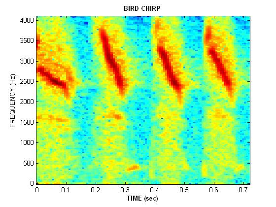
Did you notice that they all had a distinct movement of frequency vs. time.

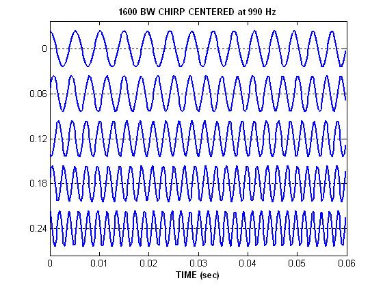
Plot Linearly Varying Chirp in the Time Domain

Let's look at one of them plotted in the time domain (i.e., \(x(t)\) vs. \(t\)). The time signal for a long LFM chirp is viewed by plotting the signal along successive rows. Each row covers 60 milliseconds, so only the first quarter of the signal is shown.

Notice how the period is getting shorter for later times.

Count the number of periods in two regions:

• for t between 0 and 10 milliseconds (the beginning of the first row)
• for t between 240 and 250 milliseconds (the beginning of the last row)
• Estimate the frequency in these two regions by taking 1/Period. Did you get 200 Hz and 500 Hz?

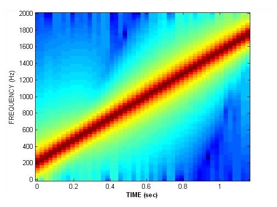
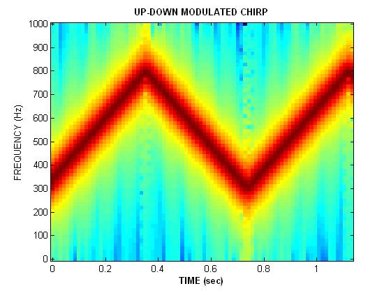
Time-frequency domain

Another way to study the sounds is to view them in the time-frequency domain. Listen to each of the signals again by clicking on the waveform.

Can you point to features in the spectrograms that correspond to the changing tones (or pitch) in the sounds your hear?

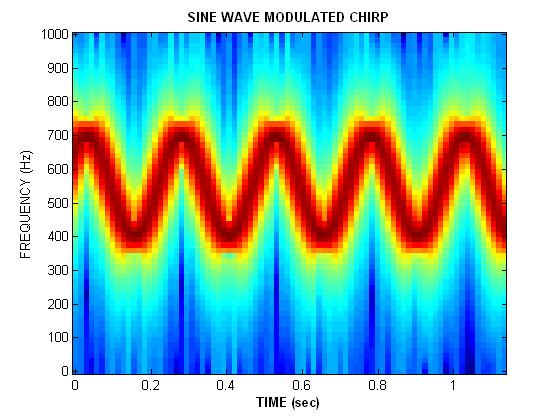
Challenge: write the mathematical formula for the sine-wave modulated chirp. Use the concept of instantaneous frequency.

How would you model the bird songs with mathematically generated synthetic chirps?

This is done by breaking the signal into many parts and computing the spectrum of each part. The spectra are plotted with a dark component representing a strong spectral component and white meaning no energy.

Instantaneous Frequency

Did you notice that all of spectra changed with time? The movement of frequency, however, is simple enough that you can describe it with a simple mathematical equation such as a straight line or a sine wave. The concept of instantaneous frequency provides the correct way to derive the frequency versus time behavior for a chirp.

Listen to the chirp with a linear frequency movement versus time .

This sound is synthesized via the formula:

$$x(t) = \cos(2\pi(m t+f)t )$$

The frequency that will be heard is determined by taking the derivative of the quantity \(2\pi(m t+f)t\) which is the argument of the cosine. If we start with \( \cos(P(t))\), the derivative must be divided by \(2\pi\) to get the frequency in Hertz.

$$f_i(t) = \frac1{2\pi} \frac{dP(t)}{dt}$$

Therefore, if \(m=5,000\) and \(f=100\), the frequency can be calculated to be $$f_i(t) = 2m t + f = 10,000 t + 100 \quad\text{(hertz)}$$

Comparison of the plot of the chirp to constant frequency sinusoids

The following example shows a comparison of the plot of the chirp to constant frequency sinusoids for reference. One way to understand the concept of instantaneous frequency is to compare the plot of a LFM chirp side-by-side with the plot of a constant frequency cosine wave. In the plot below the chirp is placed between a 300 Hz sinusoid on top and a 500 Hz sinusoid on the bottom.

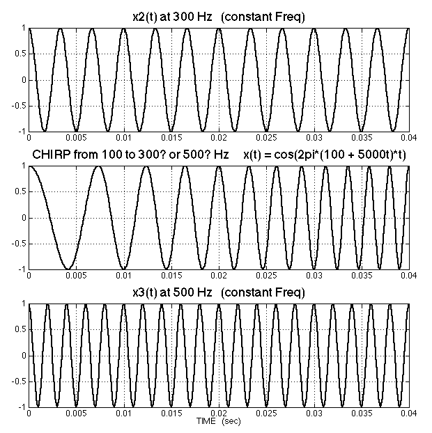
Where do the frequencies line up?

• the top plot seems to match near t = 20 milliseconds (0.02 secs).
• the bottom plot matches near t = 40 milliseconds (0.04 secs).

Thus we can conclude that the local instantaneous frequency rises linearly at a rate of 200 Hz per 20 milliseconds. As a result, the formula for instantaneous frequency versus time must be

$$f_i(t) = 10,000 t + 100 (Hertz)$$