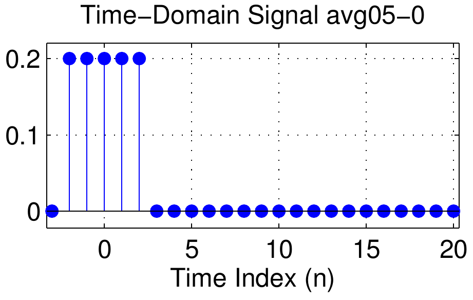
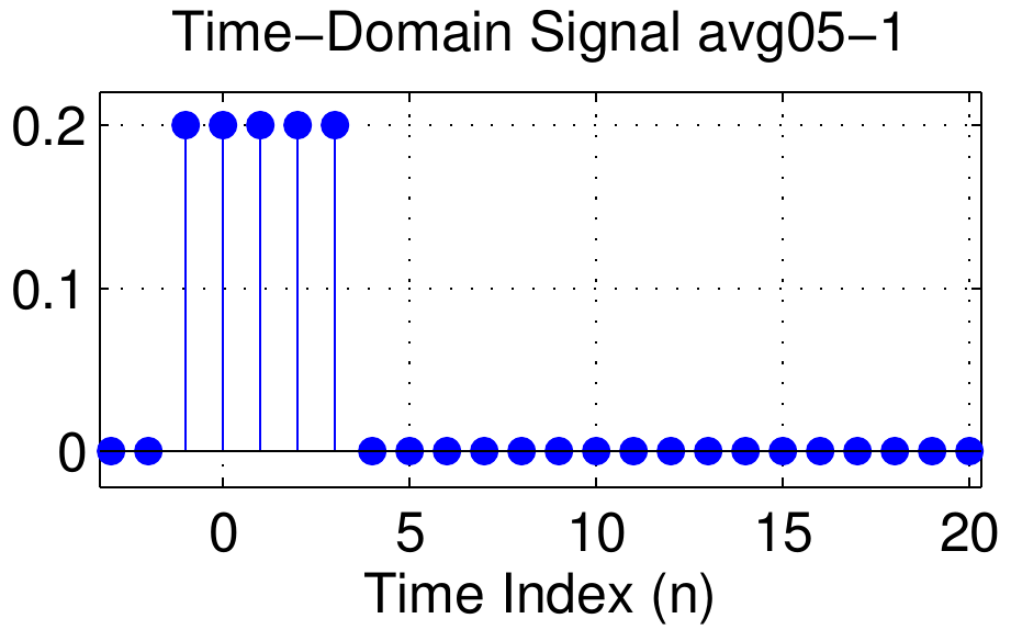
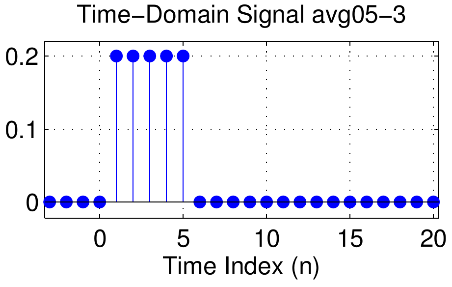
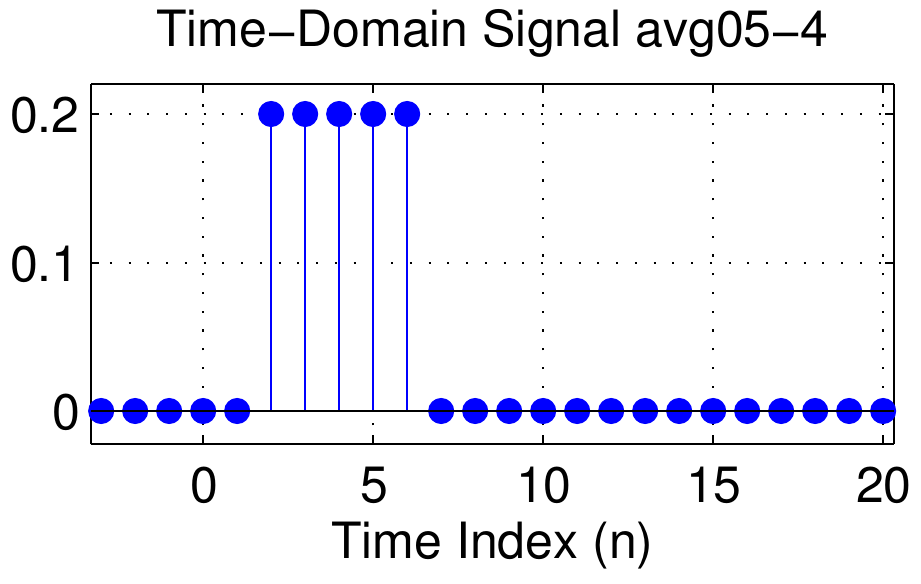
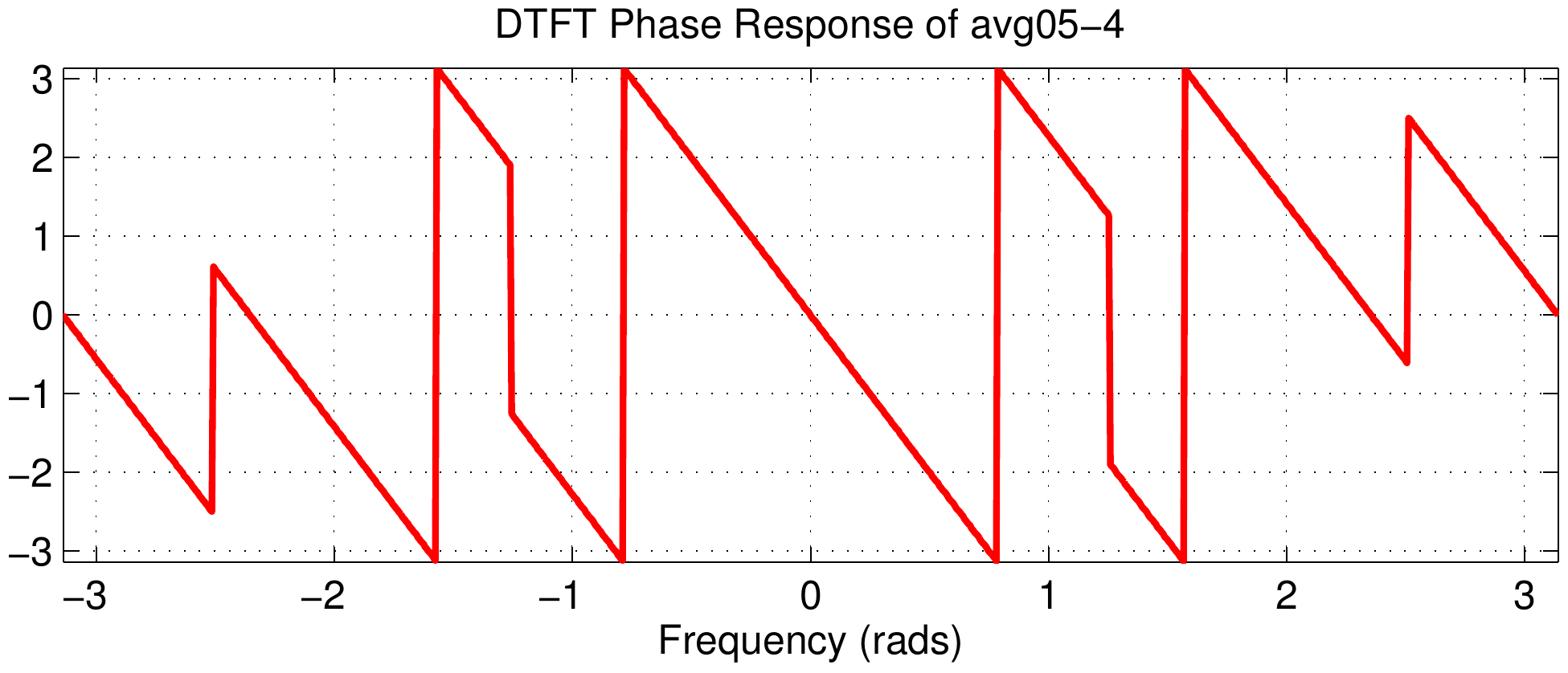
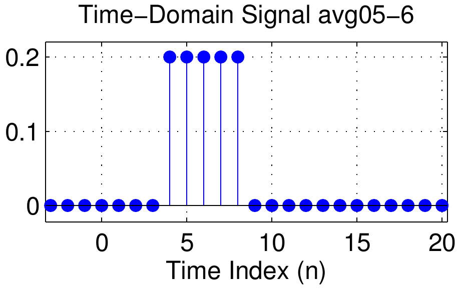
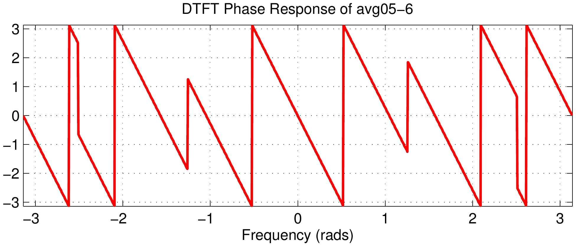
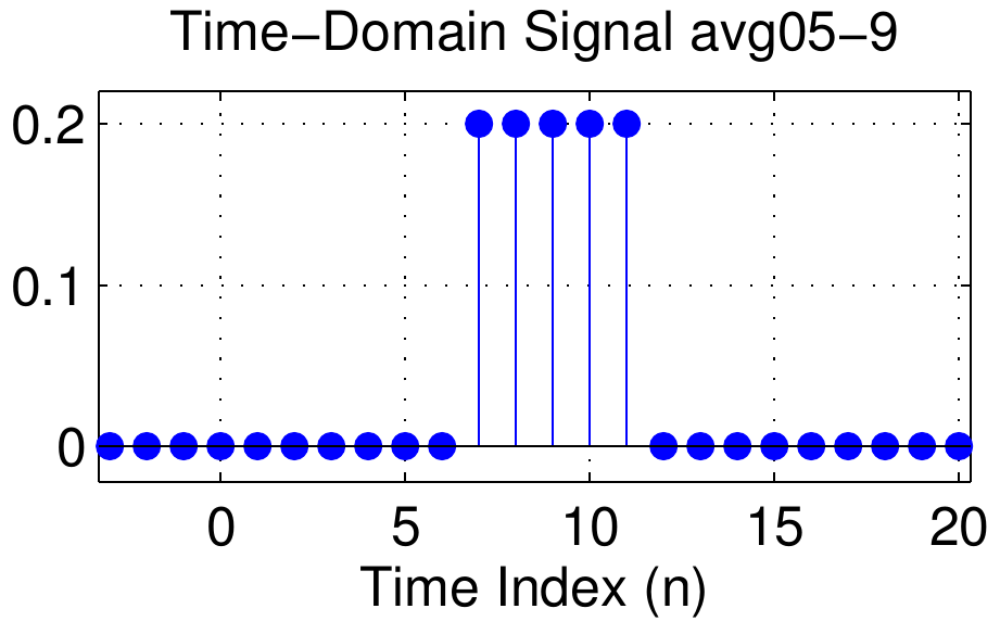
A second comparison is shown in the figure below where a length-5 pulse is time-shifted, starting at seven different indices. Going from top to bottom the length-5 pulse is shifted to the right more and more. The starting points of the signal are \(\{ -2, -1, 0, 1, 2, 4, 7\}\), but it will better to keep track of the middle of the signal, and the midpoints are \(\{ 0, 1, 2, 3, 4, 6, 9\}\). The midpoint is used to label the signals as avg05-0, avg05-1, avg05-2, and so on.

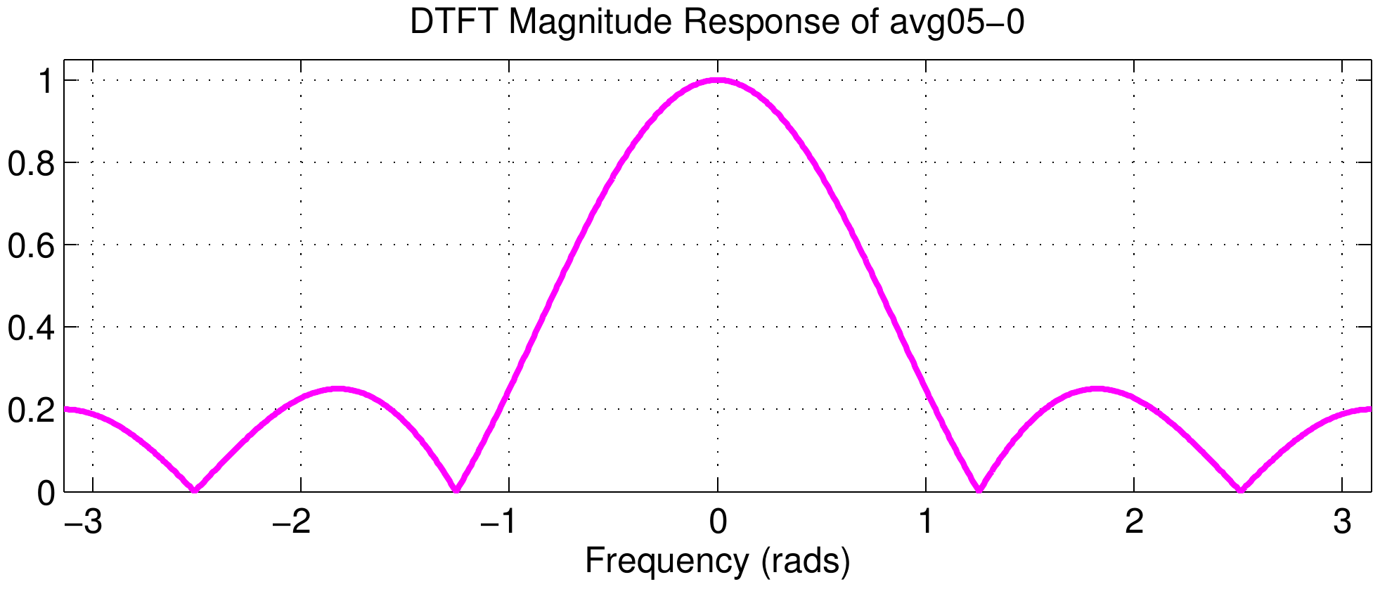
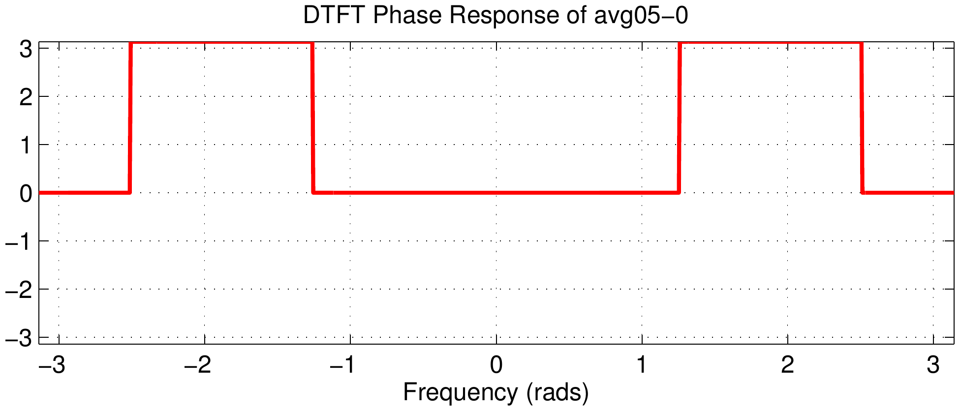
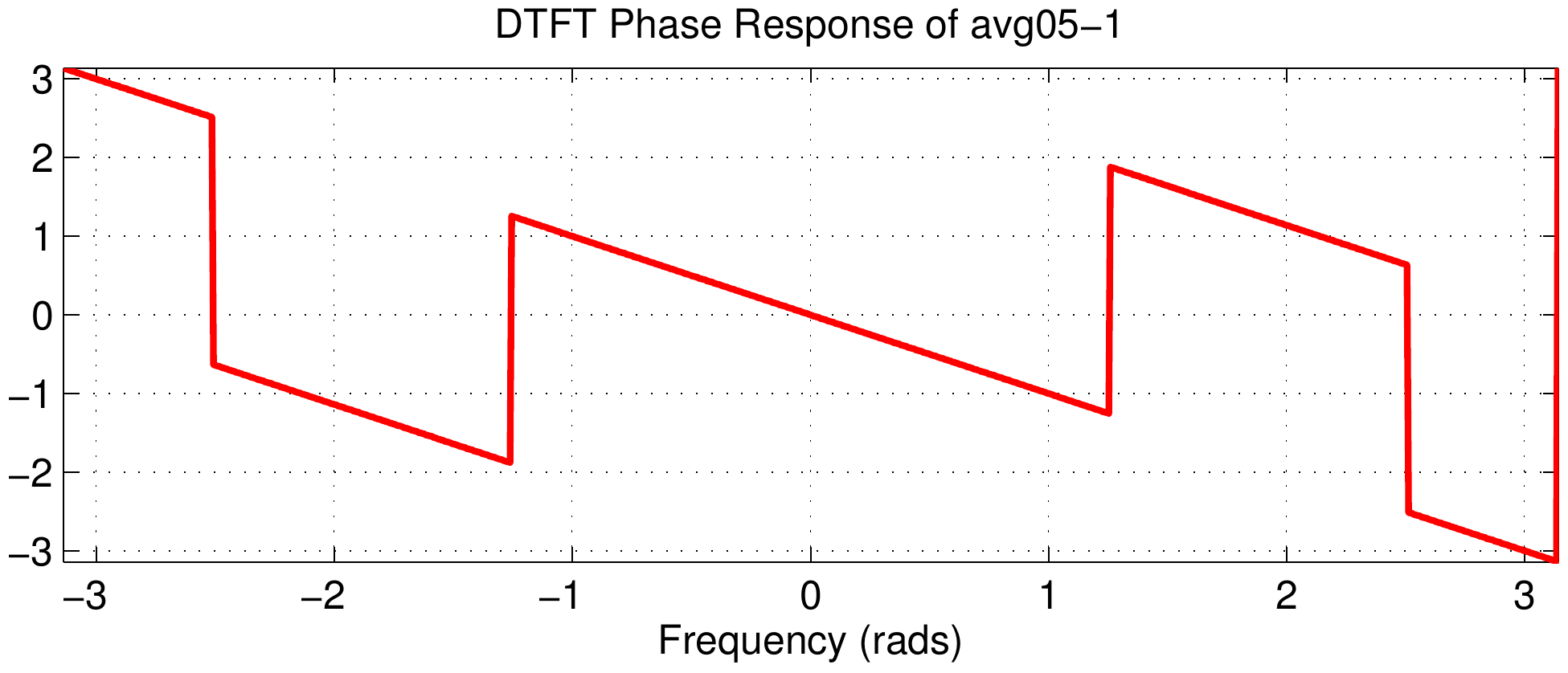
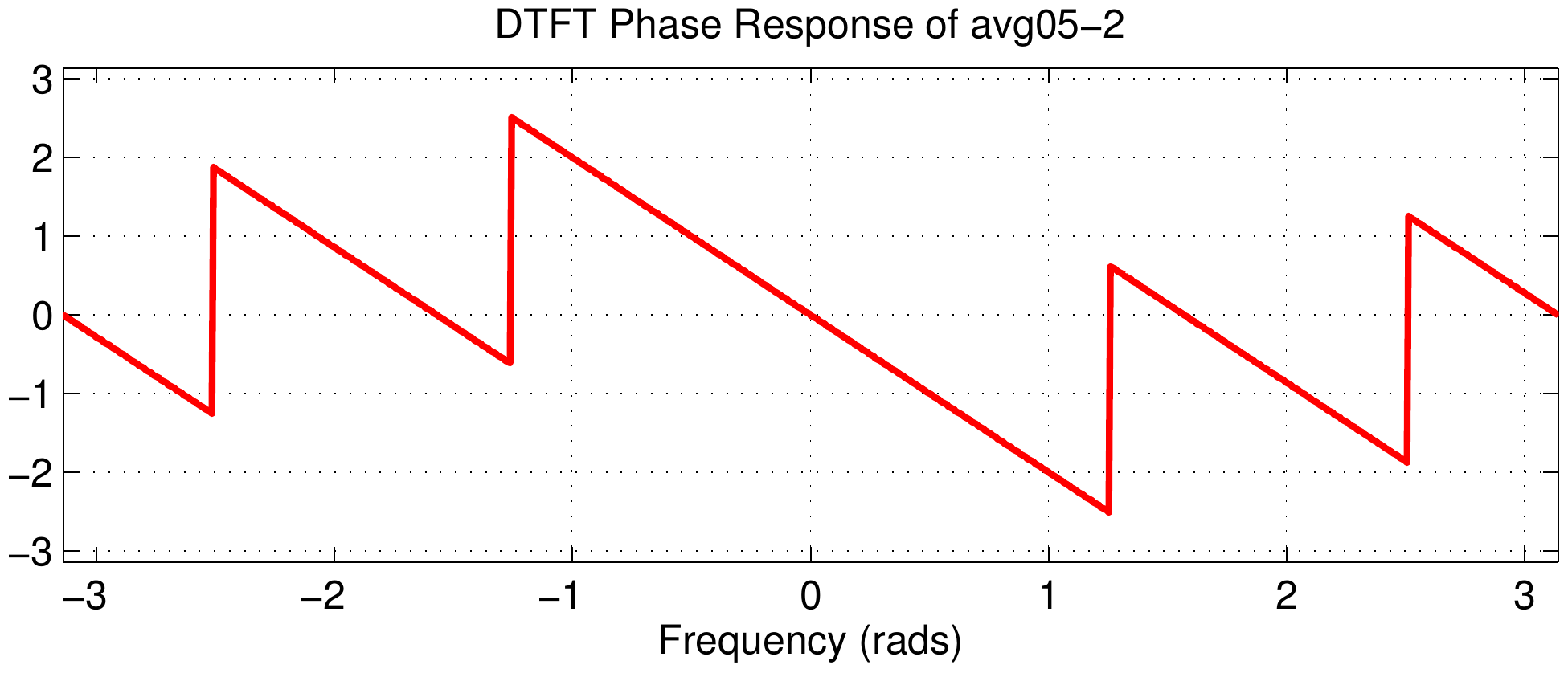
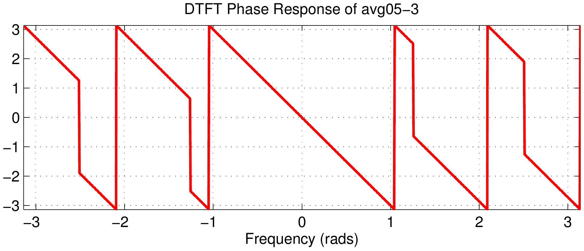
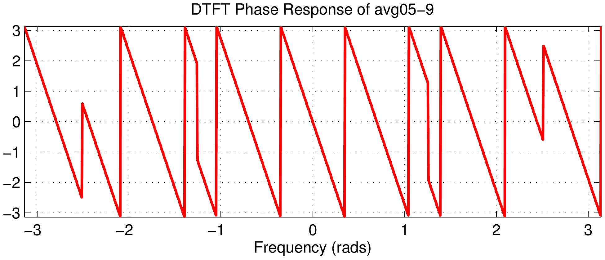
The middle column of the figure shows the DTFT magnitudes, but they are all identical because the Dirichlet component of the frequency response does not change. This can be explained by using the delay property of the DTFT $$ x[n-n_d] \quad\longleftrightarrow\quad X(e^{j\hat\omega})\ e^{-j\hat\omega n_d} $$ Multiplying by the complex exponential term will change only the phase; in terms of the phase slope the change in slope is \(-n_d\).

Therefore, looking down the third column we see that the phase slope is increasing. For the first signal (avg05-0) the phase slope is zero. This is true because that signal is symmetric about the \(n=0\) point which is where its midpoint is found. The next signal (avg05-1) has a phase slope of \(-1\) which is consistent with its delay being \(n_d=-1\) with respect to the first signal. The same logic applies to the result of the DTFT phase plots in the third column.