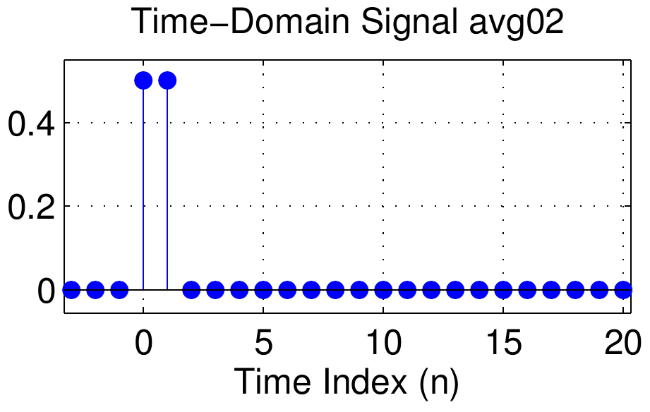
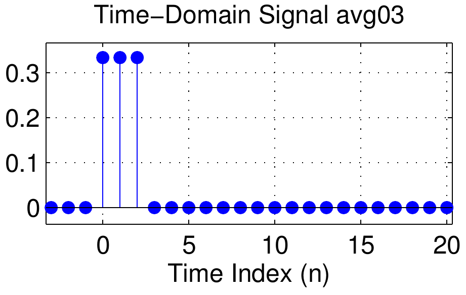
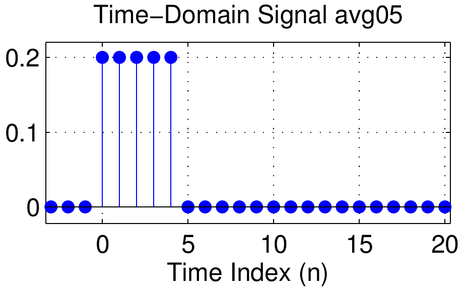
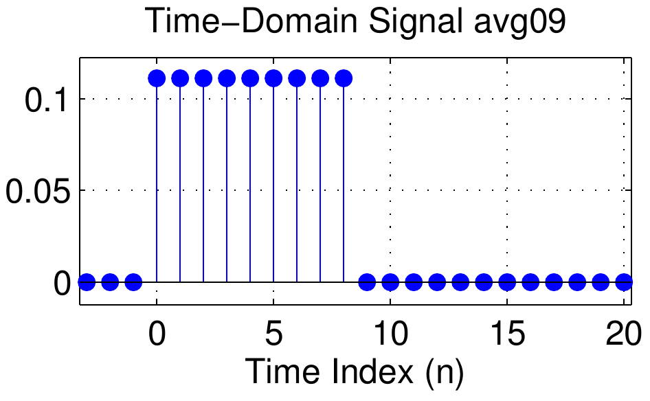
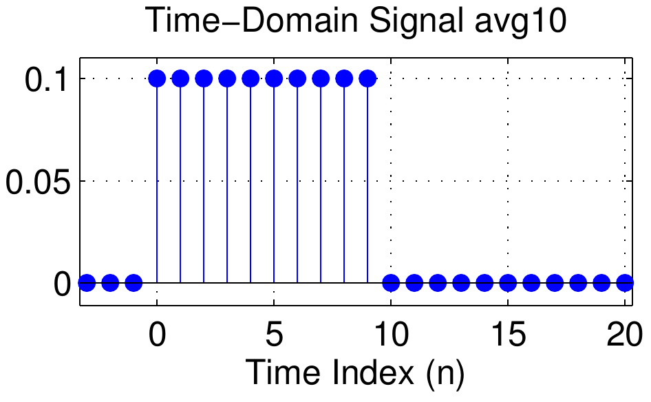
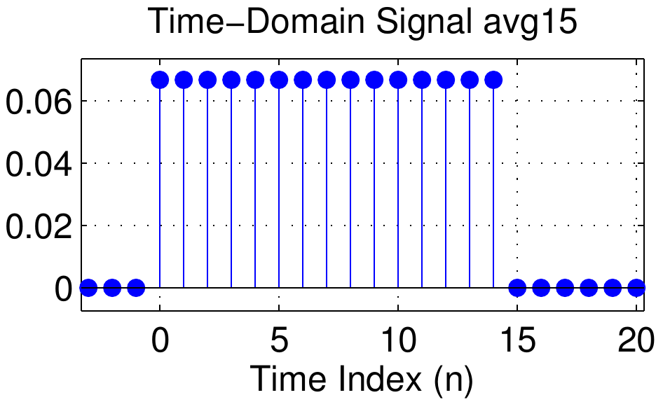
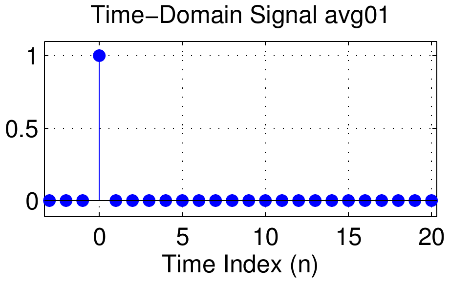
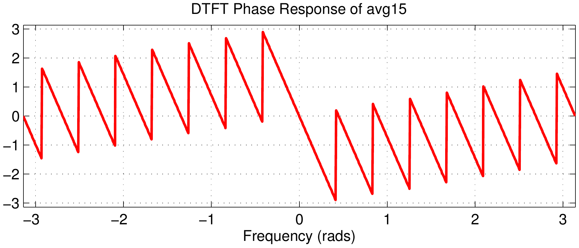
First of all, consider the family of scaled rectangular pulses shown in the left hand column of the figure below. Going from top to bottom, the length of the pulses increases. Each of the signals starts at \(n=0\) and is defined by the formula $$ x_L[n] = (1/L)(u[n] - u[n-L]) $$ where \(L\) is the length of the pulse. This signal is, in fact, the impulse response of an \(L\)-point running average filter. The signals are therefore named avg05 for the length-5 signal, avg09 for the length-9 signal, and so on.

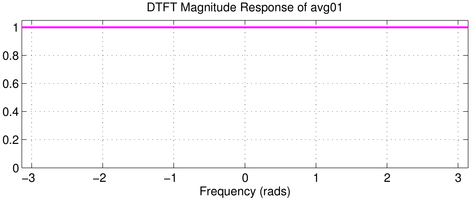
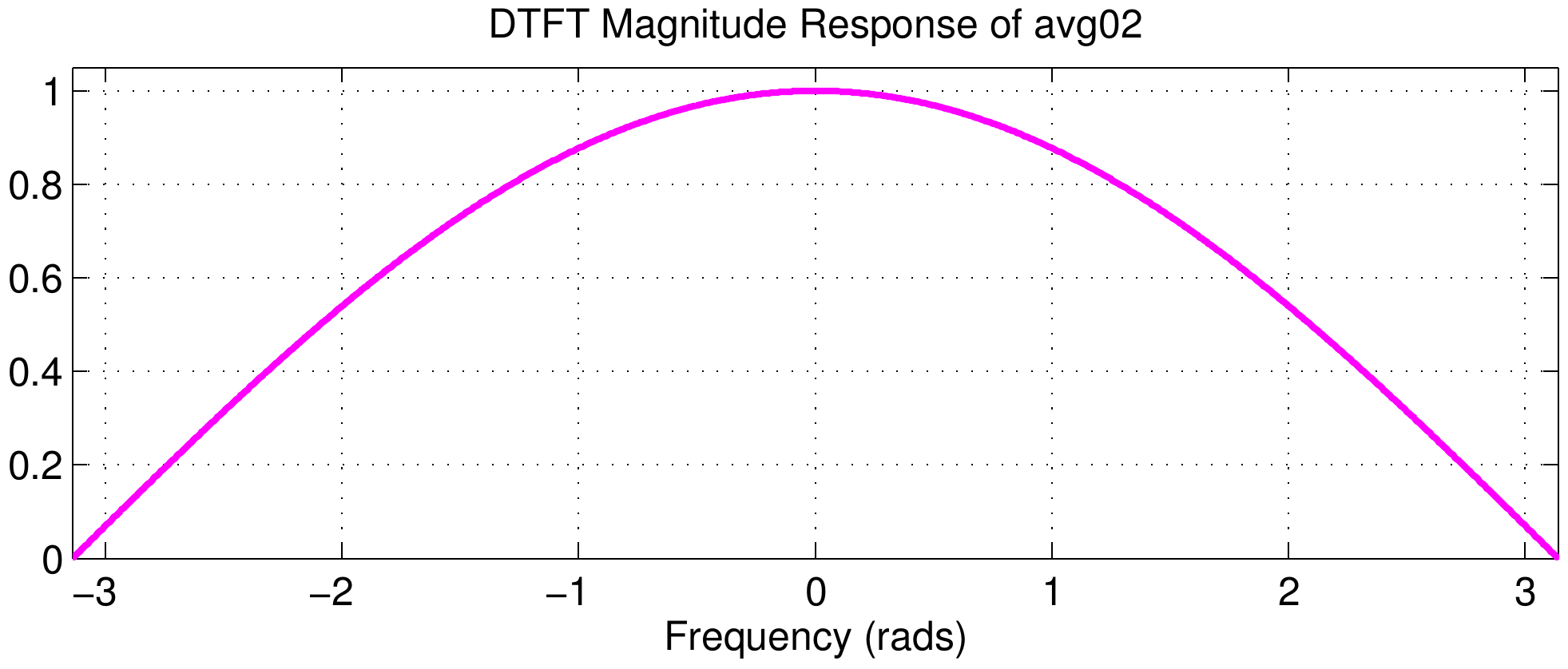
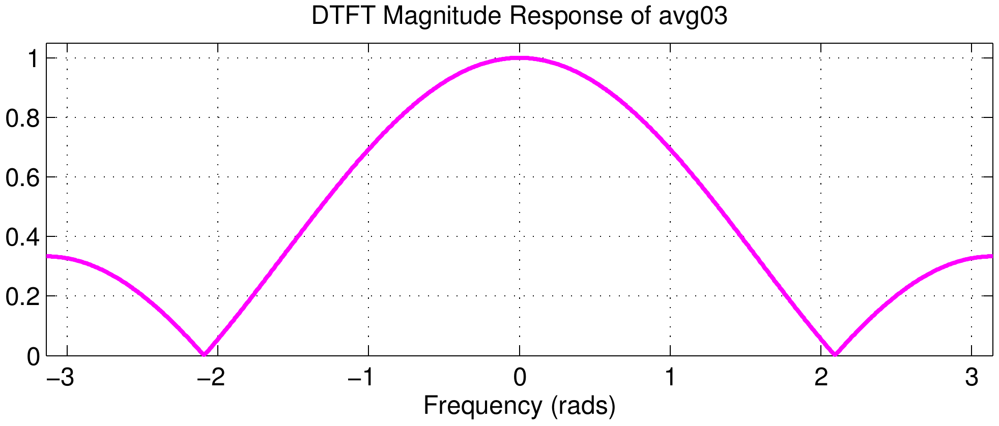
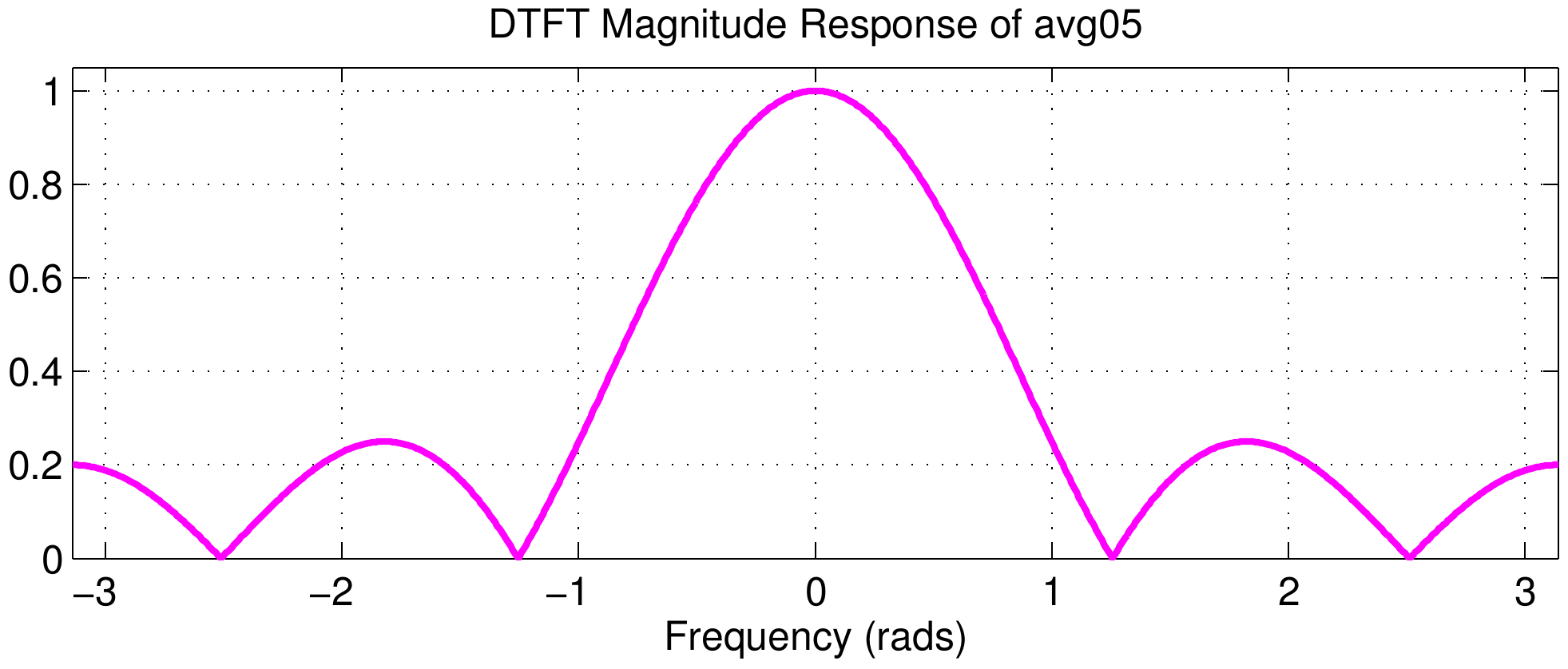
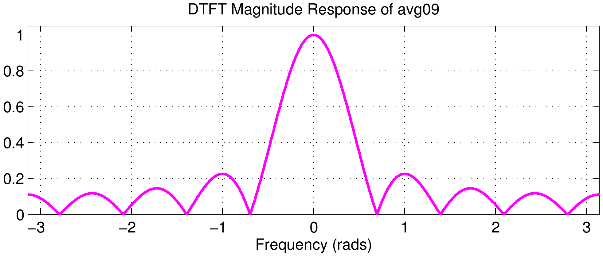
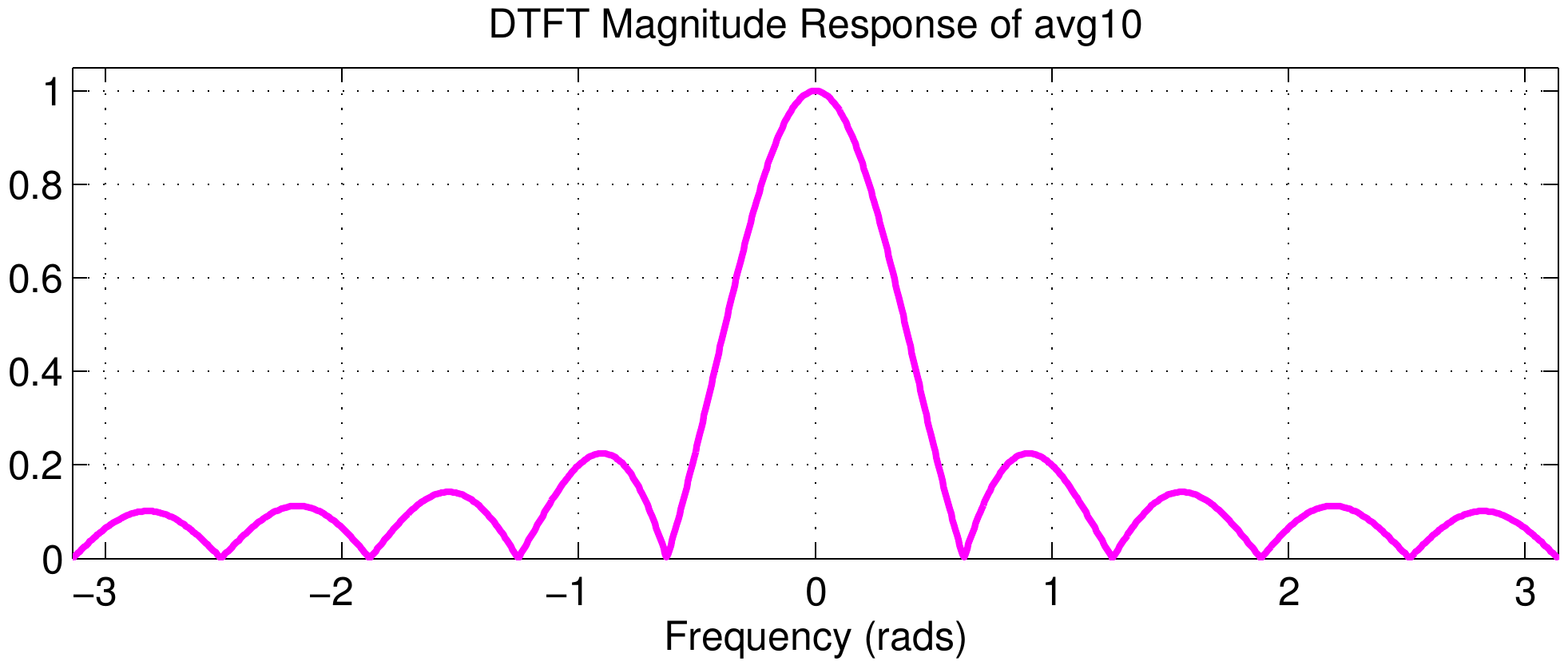
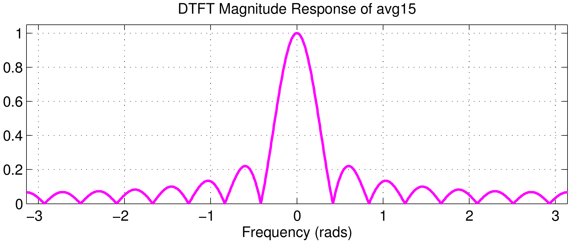
The DTFT is shown in the middle and right hand columns with the magnitude response in the middle and the phase response on the right. Going from top to bottom, the magnitude response exhibits at peak at \(\hat\omega=0\) which gets narrower as the time-domain signal gets longer. The magnitude response is zero in multiple locations, and there are more zeros as you look down the middle column. In fact, if you count the number of zeros for the length-5 signal (avg05), the result is four; for the length-9 signal, there are 8 zeros. Thus a general rule would be "the number of zeros equals the length of the rectangular pulse minus one." When the pulse length is even, the rule still holds as long as we count the zeros at \(\hat\omega=\pm \pi\) as one.

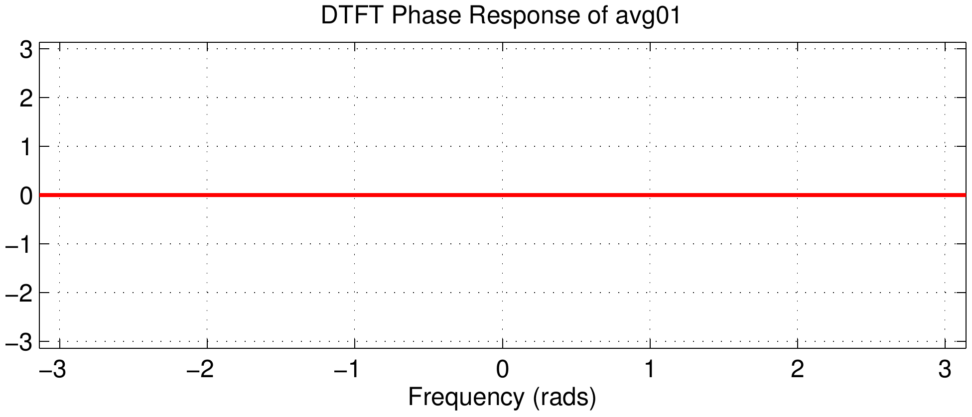
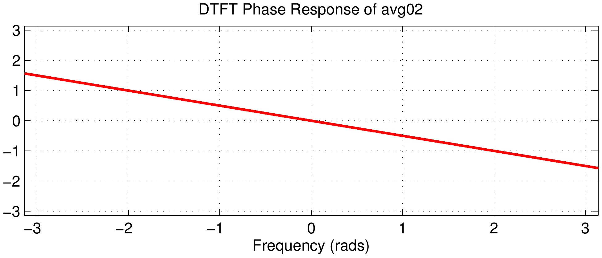
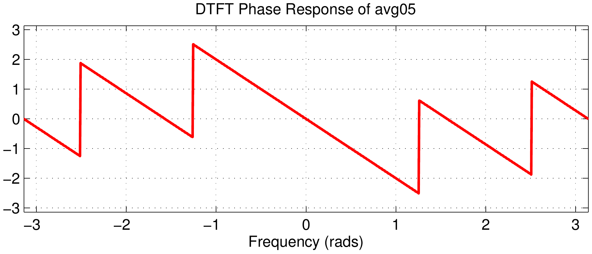
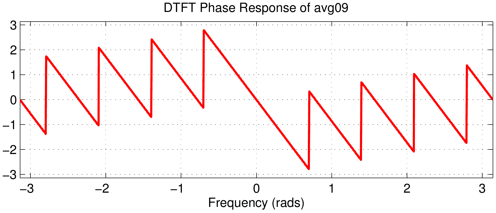
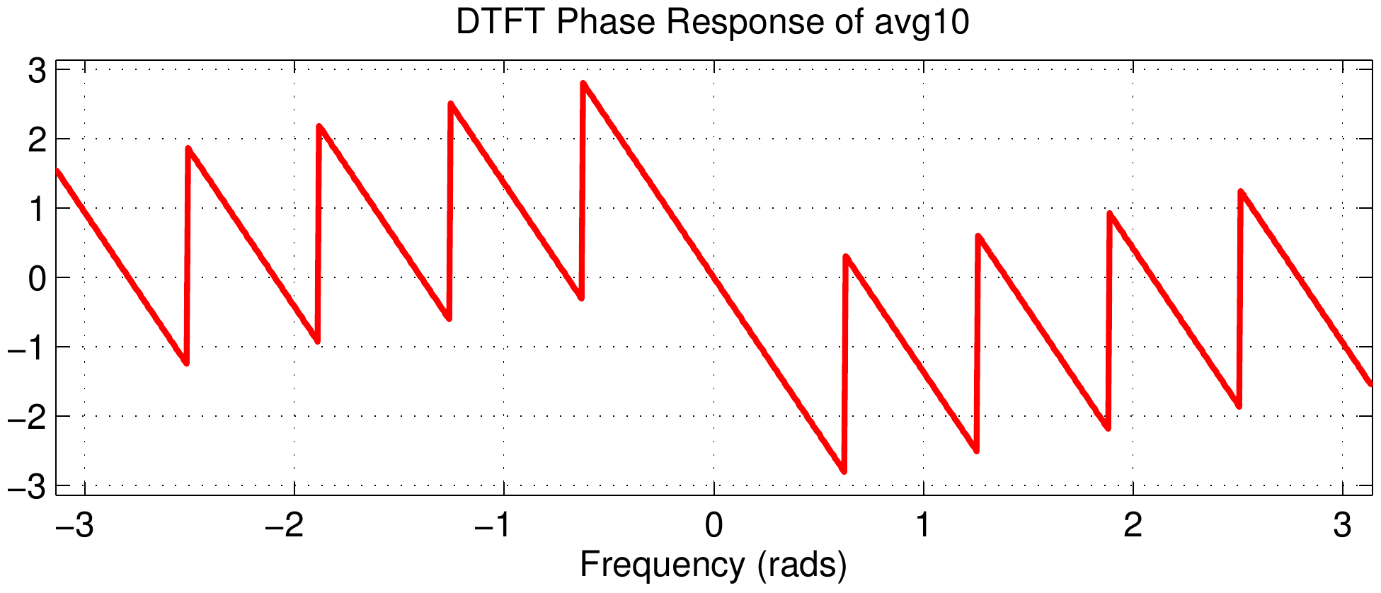
The shape of the frequency response magnitude is the absolute value of a Dirichlet form. Recall that the DTFT of the rectangular pulse is $$ X_L(e^{j\hat\omega}) = \frac{\sin(\frac{1}{2}L\hat\omega)}{\sin(\frac{1}{2}\hat\omega)}\ e^{-j\hat\omega(L-1)/2} $$ This DTFT formula shows that the phase of the DTFT changes versus frequency as \(-\hat\omega(L-1)/2\), i.e., the slope of the phase versus frequency is \(-(L-1)/2\). There is one caveat: when the Dirichlet term goes negative the phase jumps by \(\pm\pi\).

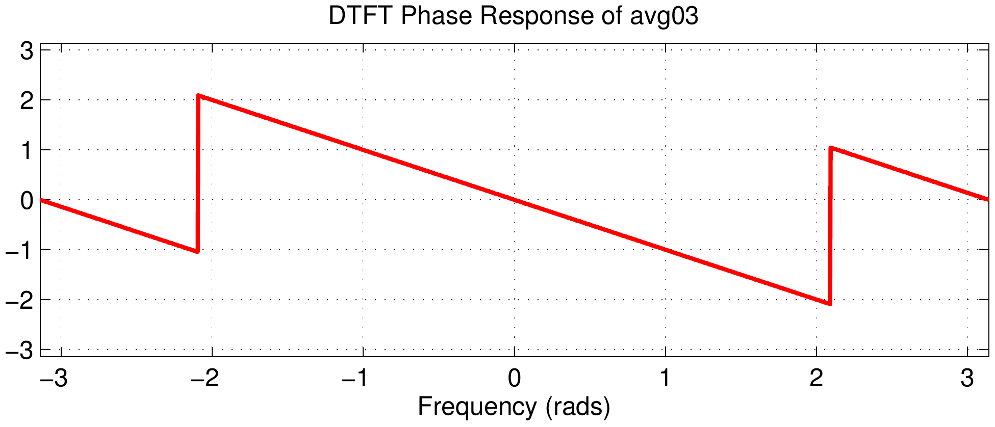
The third column shows the phase plots; going from top to bottom the slope of the linear segments of the phase becomes more and more negative. For the length-3 signal (avg03) we can measure the phase slope by noticing that the phase is zero at \(\hat\omega=0\) and is equal to \(-1\) at \(\hat\omega=1\). Equivalently, we observe that the linear segment passing through \((0,0)\) also passes through \((1,-1)\). Thus the slope is equal to \(-1\). For the case of the length-5 signal (avg05) the linear segment passing through \((0,0)\) also passes through \((1,-2)\), so the phase slope is equal to \(-2\).