Complex Numbers via MATLAB
Here we show how to
Find roots of polynomials,
Manipulate complex numbers and
Find roots of Unity.
zvect plots each vector with it's tail at the origin.
zcat plots each vector head to tail.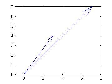
You might want to use the axis command to put 0,0 in the center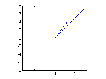
Do you see a relationship between the power to which z is raised and the number of vectors?
What if we solve \(z^{10}=1\)?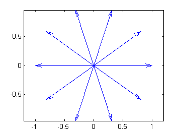
Did you guess right?
Finding roots of polynomials
MATLAB can find the roots of polynomials via the roots command. To find the roots of \(z^2+6z+25\) you enter the coefficients of \(z\)
>>eqn = [1 6 25]
eqn =
     1     6    25
and ask for the roots:
>>roots(eqn)
ans =
  -3.0000 + 4.0000i
  -3.0000 - 4.0000i
Notice that this is the same answer as given in the book.
MATLAB outputs \(i\) as the square root of \(-1\), but
you can use \(j\) too.
Manipulating complex numbers
There are many commands for manipulating complex numbers.
You can guess what they do by their names.
>>z = 3 + j*4
z =
   3.0000 + 4.0000i
>>real(z)
ans =
     3
>>imag(z)
ans =
     4
>>conj(z)
ans =
   3.0000 - 4.0000i
>>abs(z)
ans =
     5
>>angle(z)
ans =
    0.9273
Note the angle is in radians, you can convert to degrees by:
>>angle(z)*180/pi
ans =
   53.1301
If you want to input as polar use:
>>z2=10*exp(j*pi/4)
z2 =
   7.0711 + 7.0711i
or
>>10*exp(j*45/180*pi)
ans =
   7.0711 + 7.0711i
A handy way to see a complex number in several forms is zprint. zprint is not part of MATLAB, but comes with this CD-ROM
>>zprint([z,z2])
 Z =     X    +     jY     Magnitude    Phase    Ph/pi   Ph(deg)
           3           4           5    0.927    0.295    53.13
       7.071       7.071          10    0.785    0.250    45.00
Type help zprint for more details
Plotting vectors
You can plot the two vectors (z and z2) via zvect and zcat.zvect plots each vector with it's tail at the origin.
zcat plots each vector head to tail.
zvect([z, z2])
zcat([z, z2])
You might want to use the axis command to put 0,0 in the center
zvect([z, z2])
axis([-8 8 -8 8])
The example from section 2.4.1 via MATLAB is:
>>z1 = 7*exp(j*4*pi/7)
z1 =
  -1.5576 + 6.8245i
>>z2 = 5*exp(-j*5*pi/11)
z2 =
   0.7116 - 4.9491i
Notice MATLAB automatically converts them to rectangular form. Now just add them.
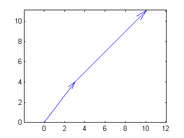
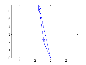
>>z3 = z1 + z2
z3 =
  -0.8461 + 1.8754i
We can also show this graphically with:
>>zcat([z1, z2]), hold on
>>zvect(z3)
Finding roots of Unity
We know that the square root of \(1\) gives two answers, \(+1\) and \(-1\). Likewise, for the \(n\)-th root of \(1\), we get \(n\) answers. Here we find the third roots of unity, by solving \(z^3=1\)
>>p = [1 0 0 -1]
p =
     1     0     0    -1
>>z = roots(p)
z =
  -0.5000 + 0.8660i
  -0.5000 - 0.8660i
   1.0000
You can check to see if you have the right polynomial with the
poly2sym command.
>>poly2sym(p,'z')
ans =
z^3-1
Good, it checks.
We might see a pattern if we convert to polar.
>>zprint(z)
 Z =     X    +     jY     Magnitude    Phase    Ph/pi   Ph(deg)
        -0.5       0.866           1    2.094    0.667   120.00
        -0.5      -0.866           1   -2.094   -0.667  -120.00
           1           0           1    0.000    0.000     0.00
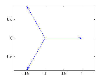
Hmmm, do you see the pattern? Let's plot them.
zvect(z)
Do you see a relationship between the power to which z is raised and the number of vectors?
What if we solve \(z^{10}=1\)?
>>z10 = roots([1 0 0 0 0 0 0 0 0 0 -1])
zvect(z10)
z10 =
  -1.0000
  -0.8090 + 0.5878i
  -0.8090 - 0.5878i
  -0.3090 + 0.9511i
  -0.3090 - 0.9511i
   0.3090 + 0.9511i
   0.3090 - 0.9511i
   1.0000
   0.8090 + 0.5878i
   0.8090 - 0.5878i
>>zprint(z10)
 Z =     X    +     jY     Magnitude    Phase    Ph/pi   Ph(deg)
          -1           0           1    3.142    1.000   180.00
      -0.809      0.5878           1    2.513    0.800   144.00
      -0.809     -0.5878           1   -2.513   -0.800  -144.00
      -0.309      0.9511           1    1.885    0.600   108.00
      -0.309     -0.9511           1   -1.885   -0.600  -108.00
       0.309      0.9511           1    1.257    0.400    72.00
       0.309     -0.9511           1   -1.257   -0.400   -72.00
           1           0           1    0.000    0.000     0.00
       0.809      0.5878           1    0.628    0.200    36.00
       0.809     -0.5878           1   -0.628   -0.200   -36.00
>>zvect(z10)
Did you guess right?
 DSP First 2e
McClellan, Schafer, Yoder
ISBN-10: 0136019250 • ISBN-13: 9780136019251
© 2016 Pearson Education, Inc.