DSP FIRST 2e
10. IIR Filters
–
Problems with selected Solutions
198
10
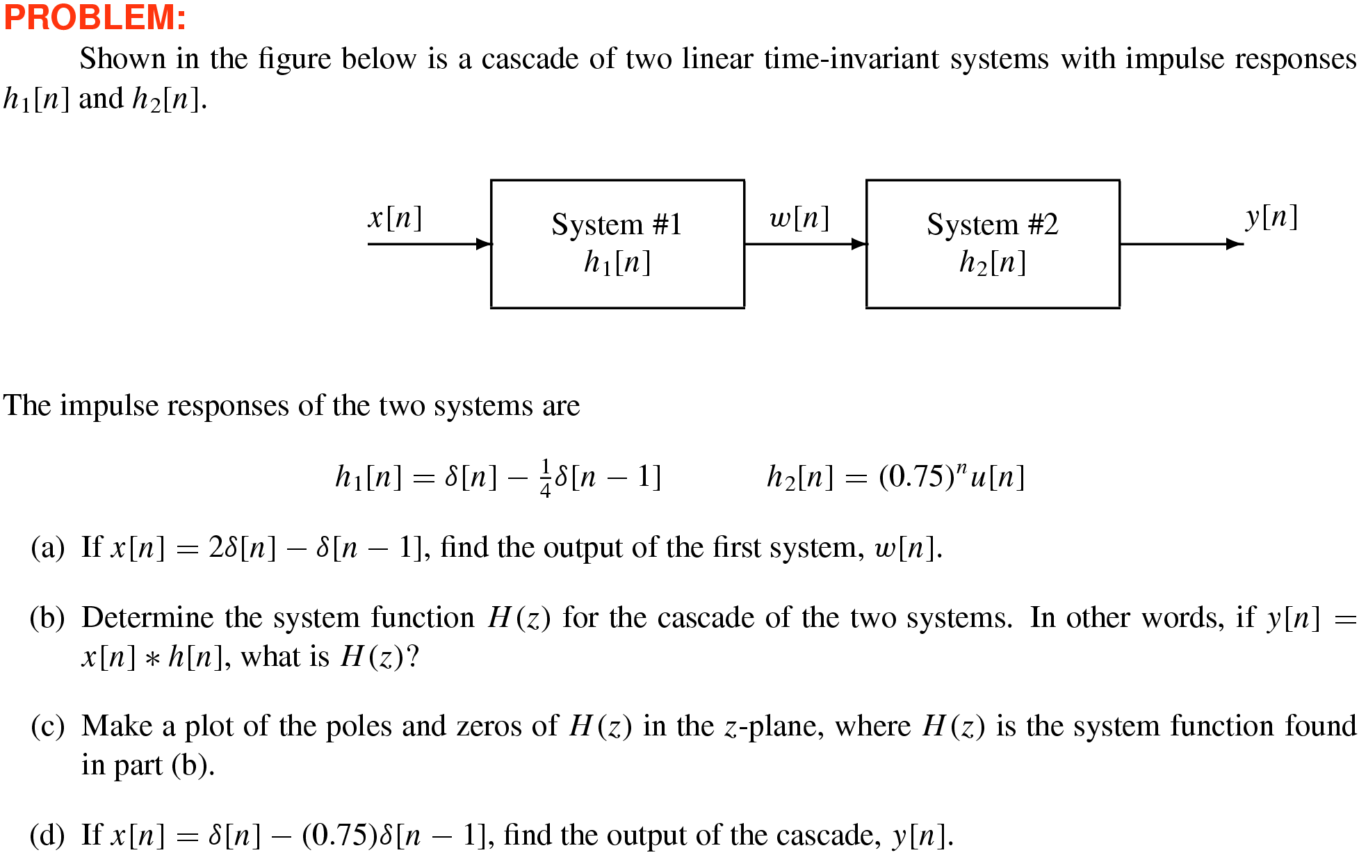
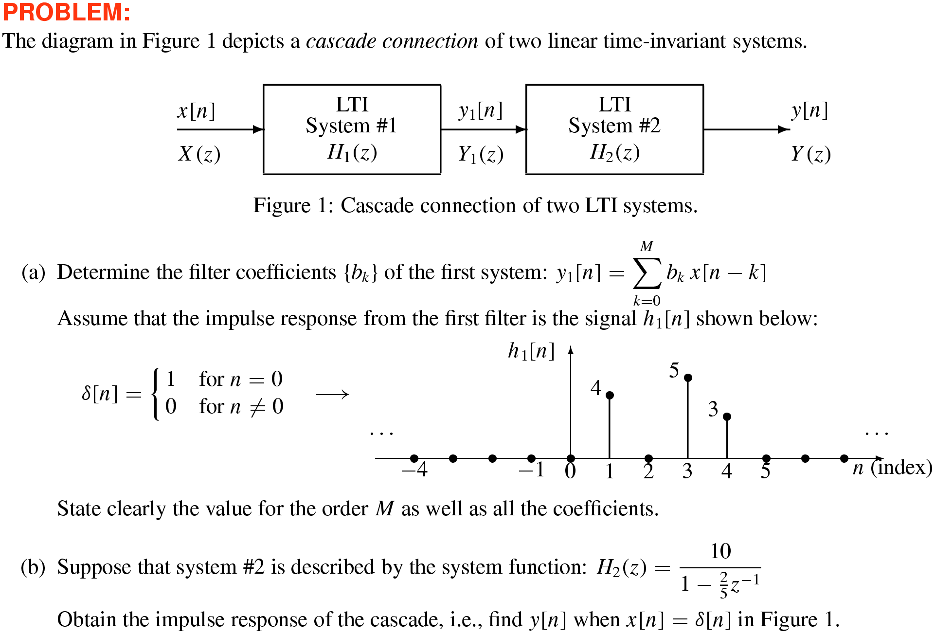
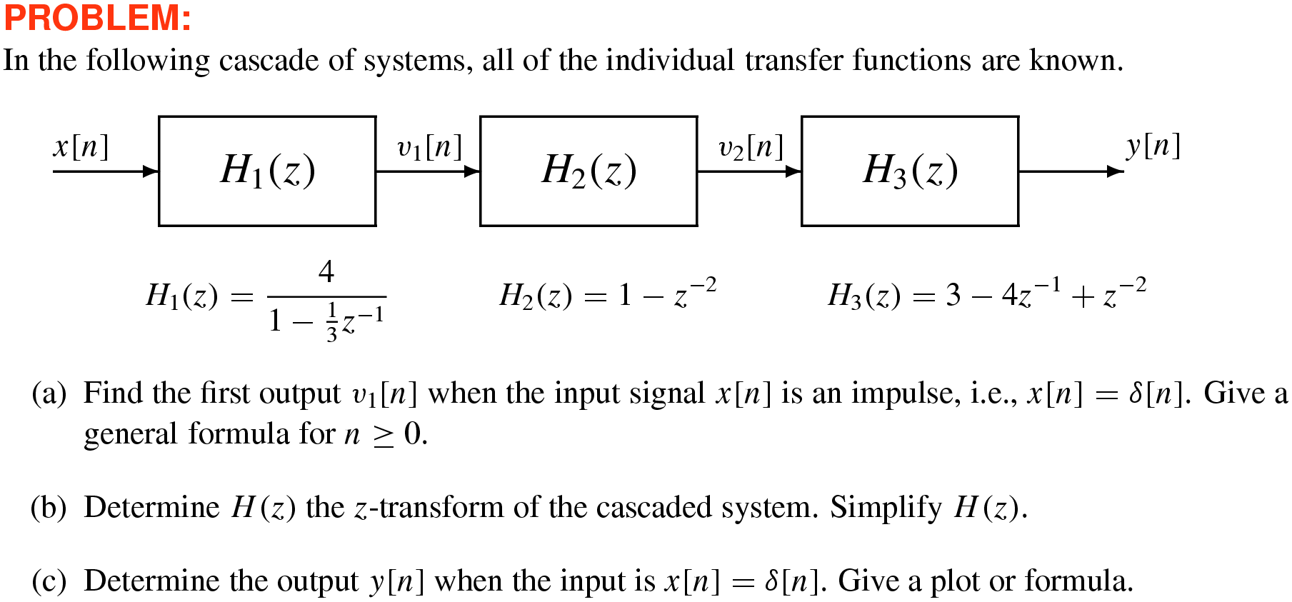
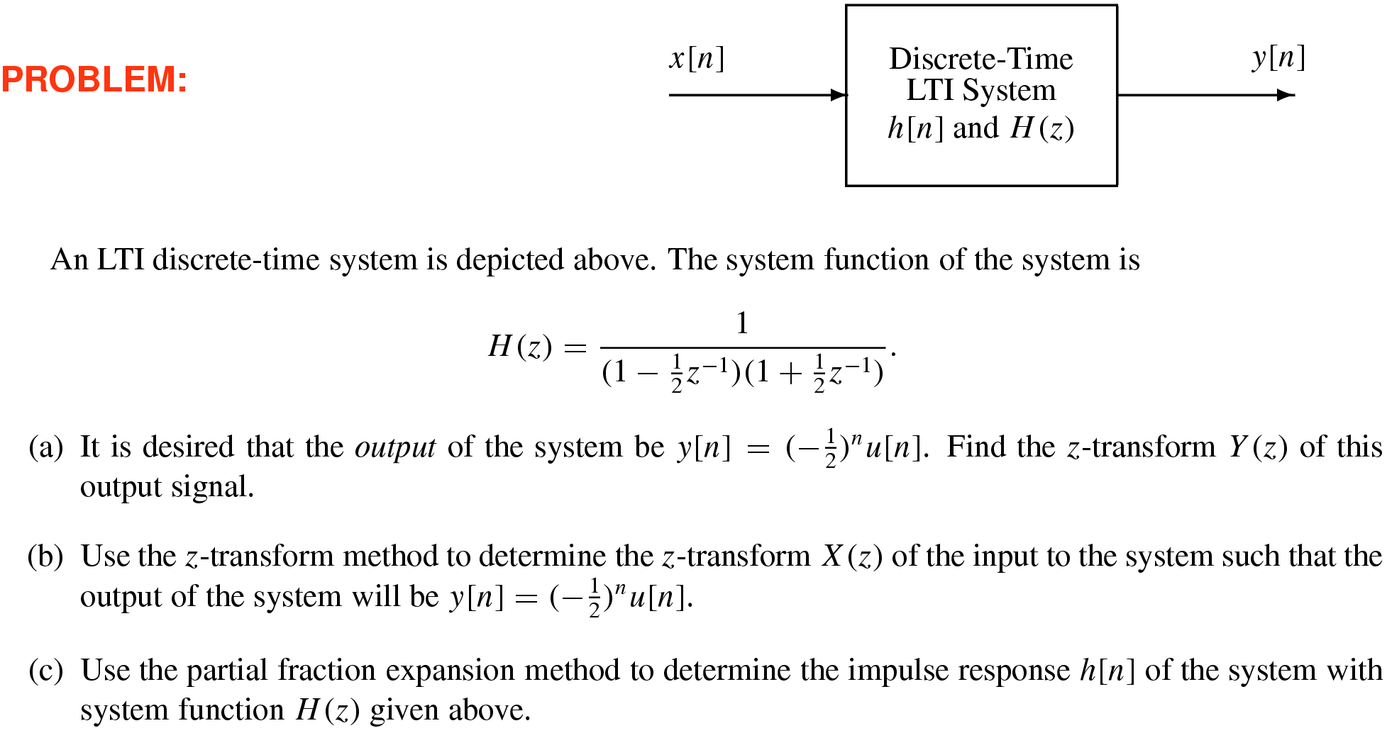
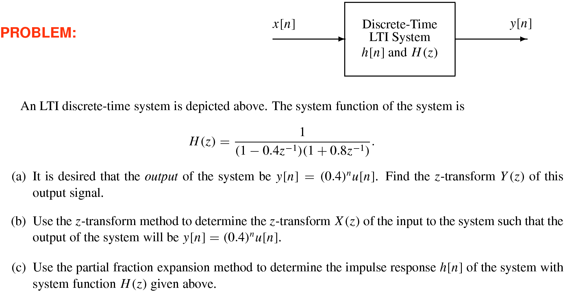
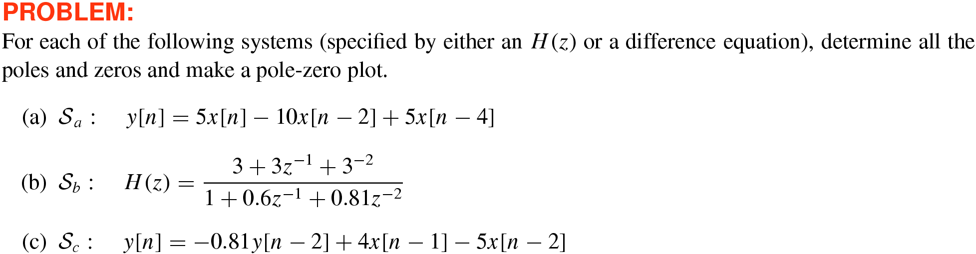
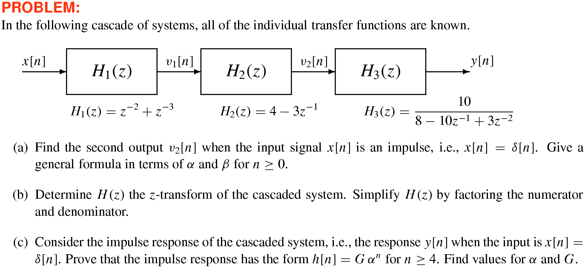
–1 Impulse response and \(H(z)\) for cascade
10
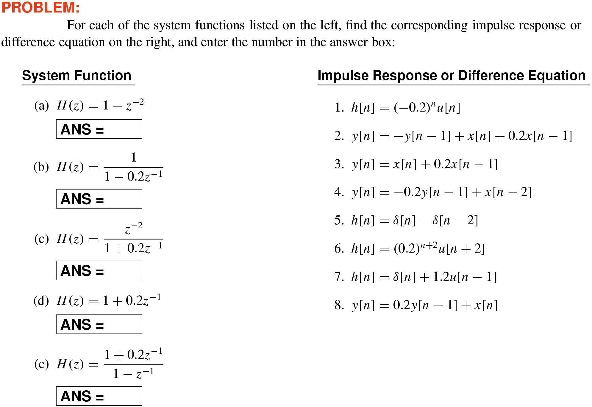
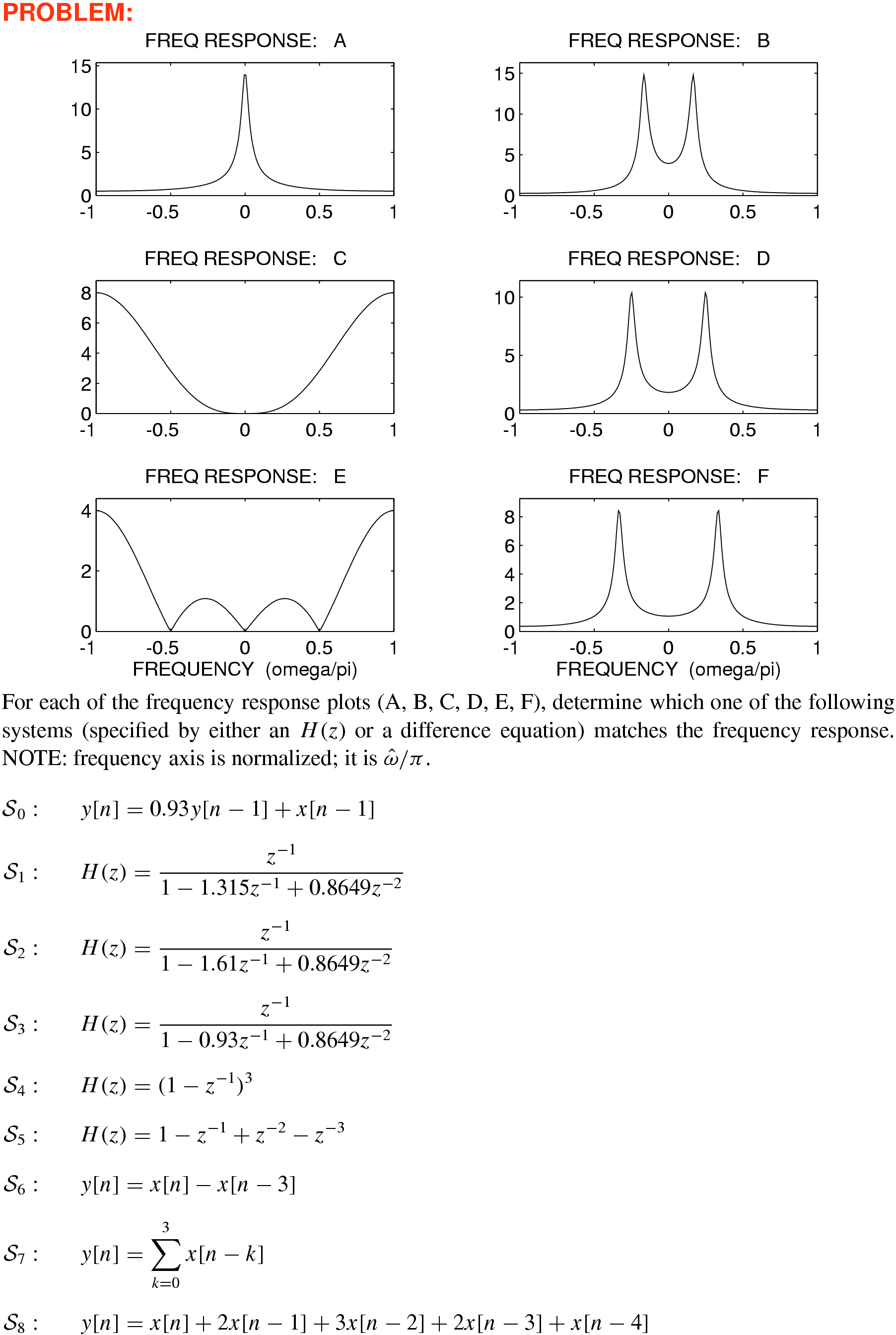
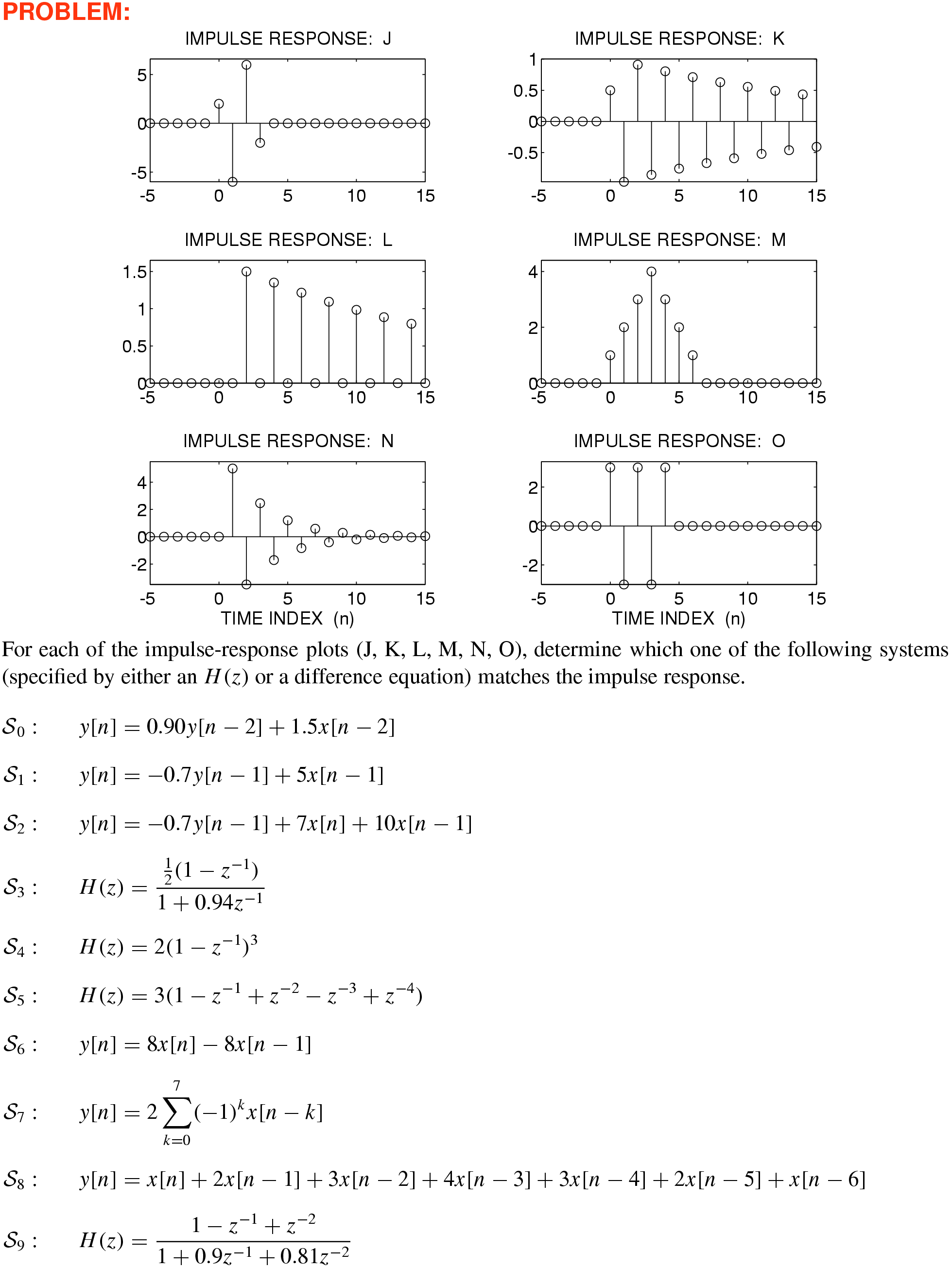
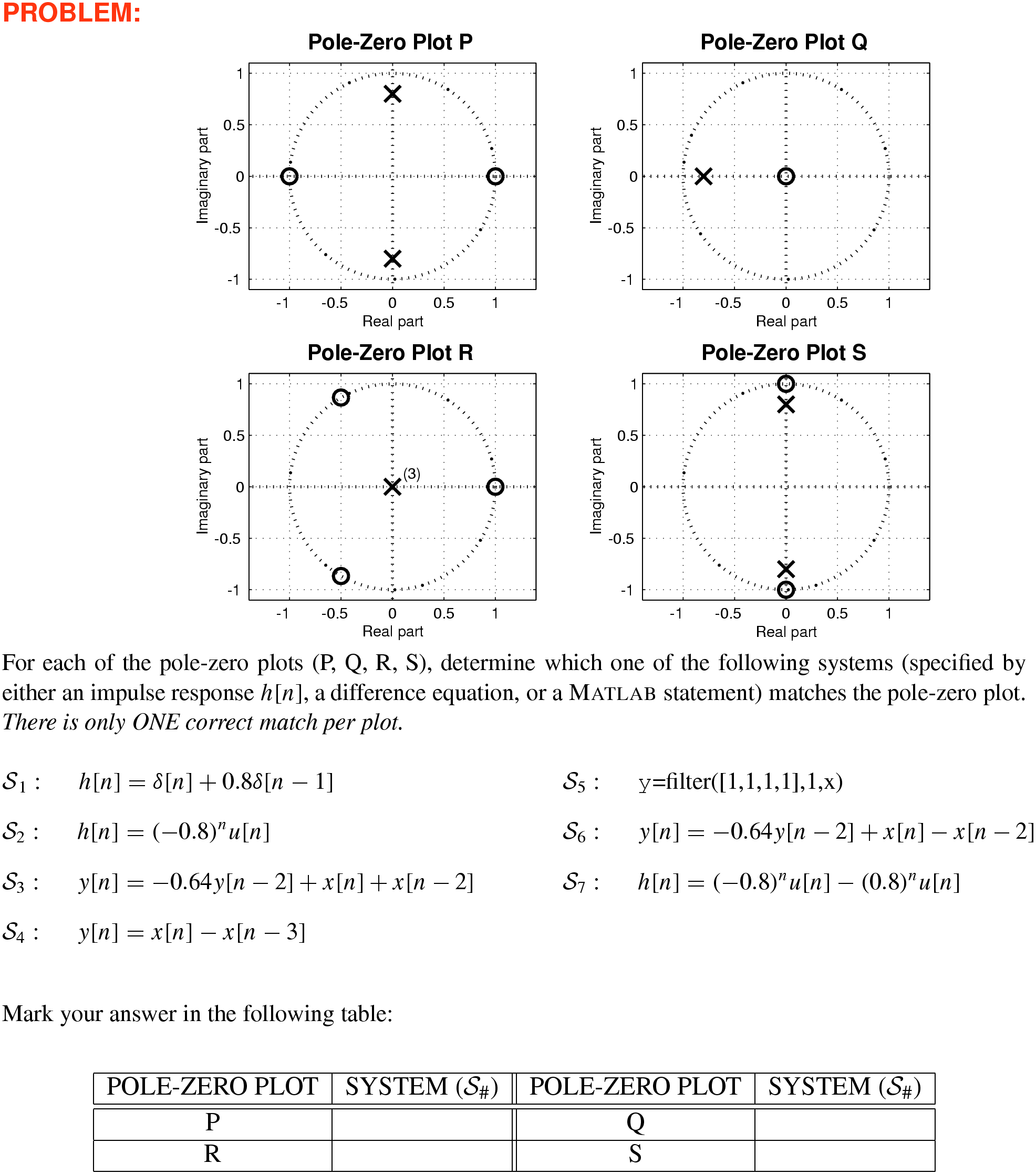
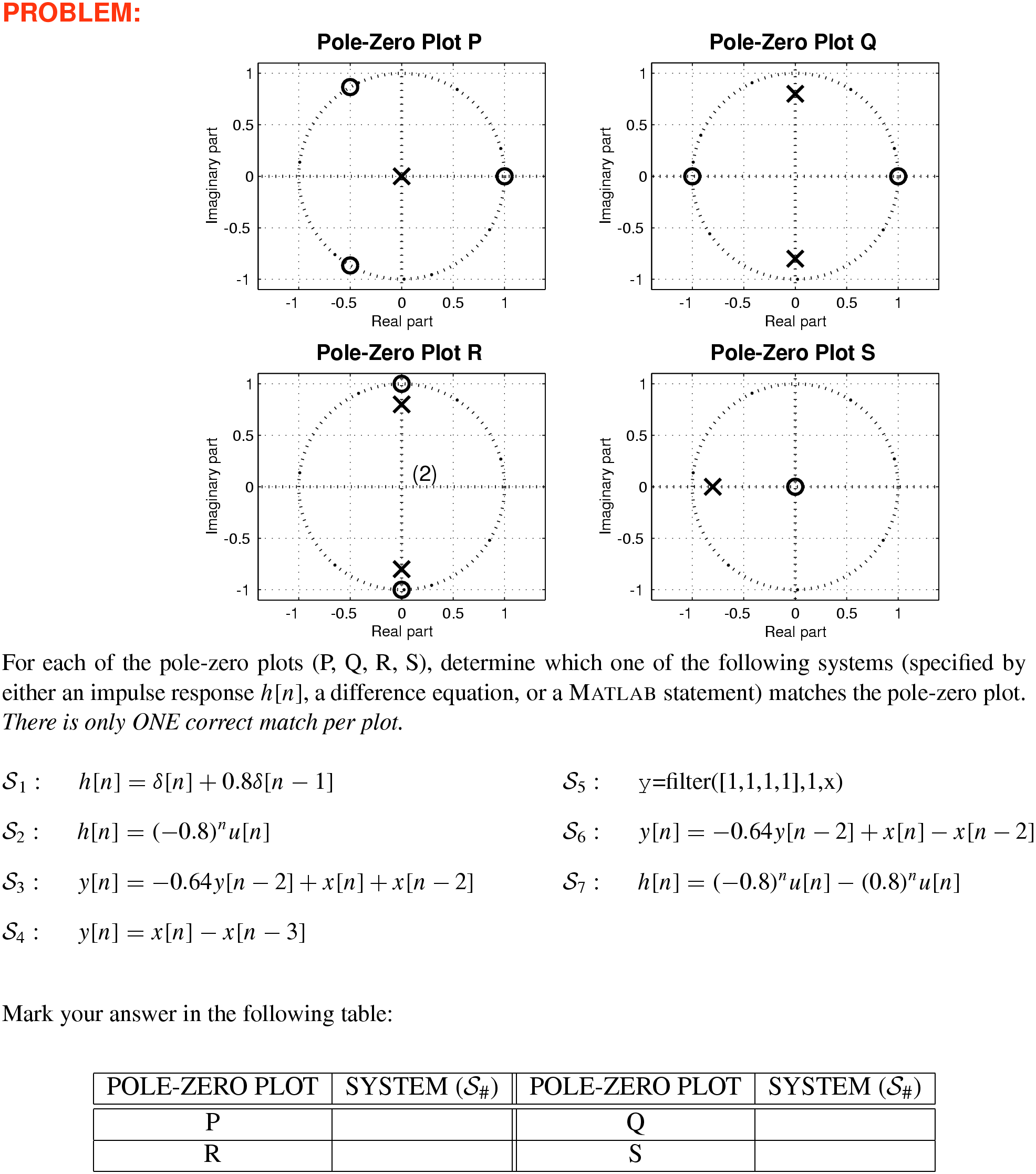
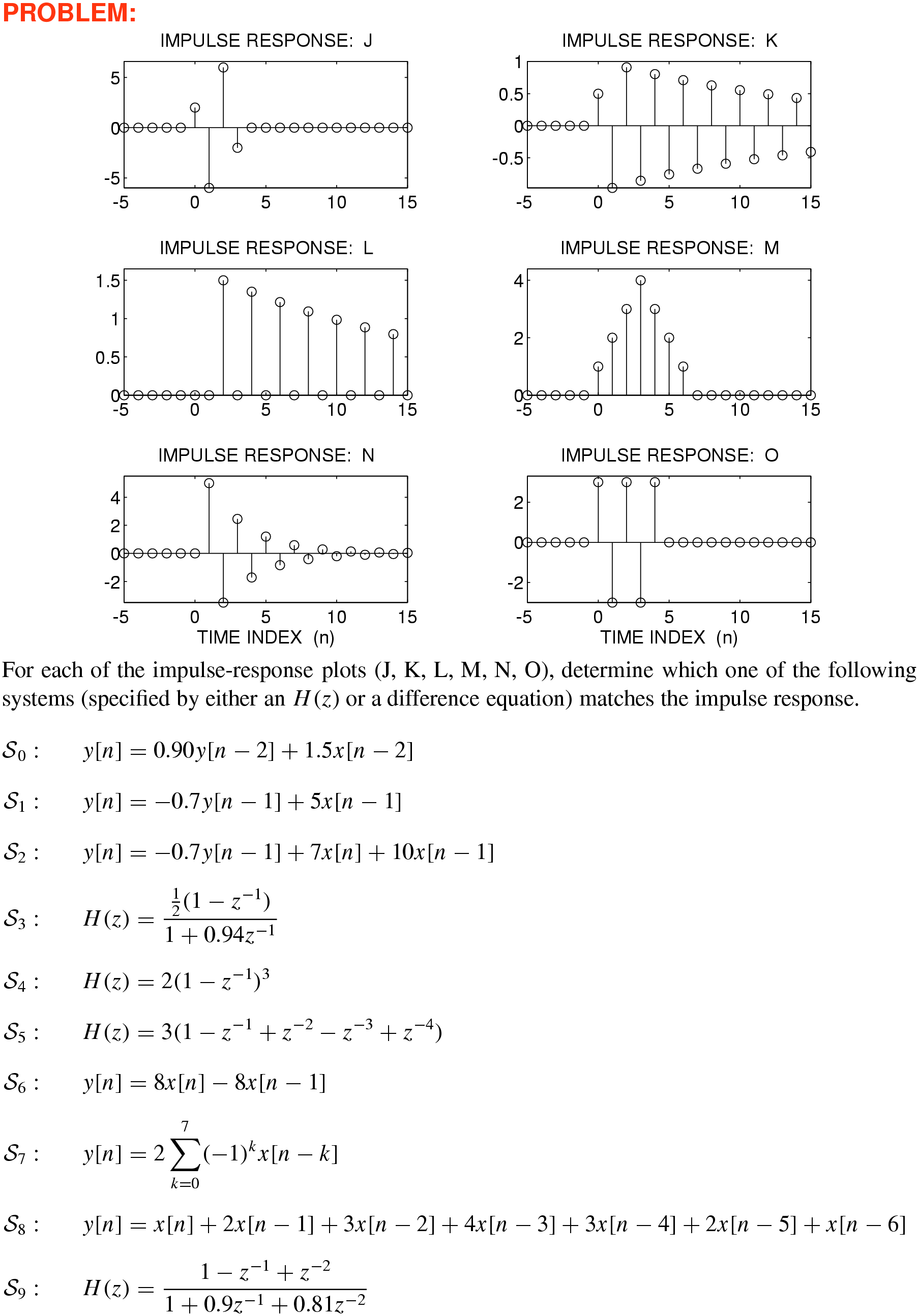
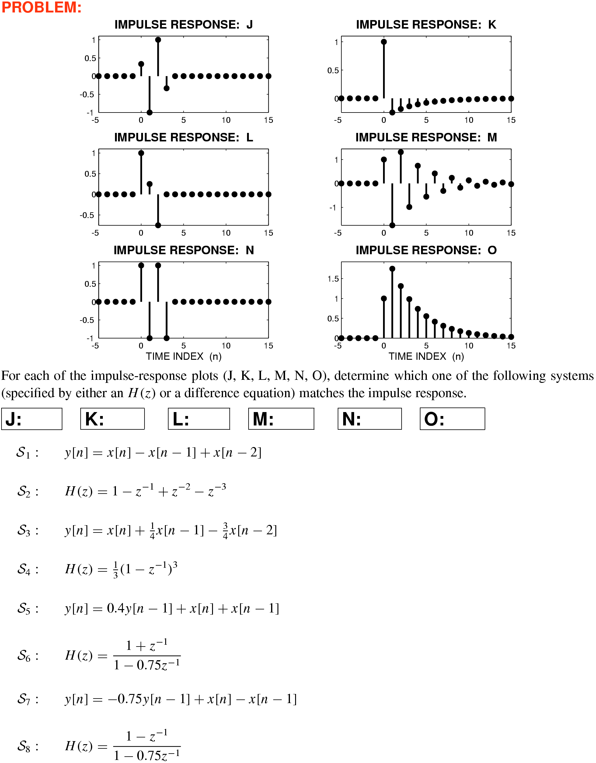
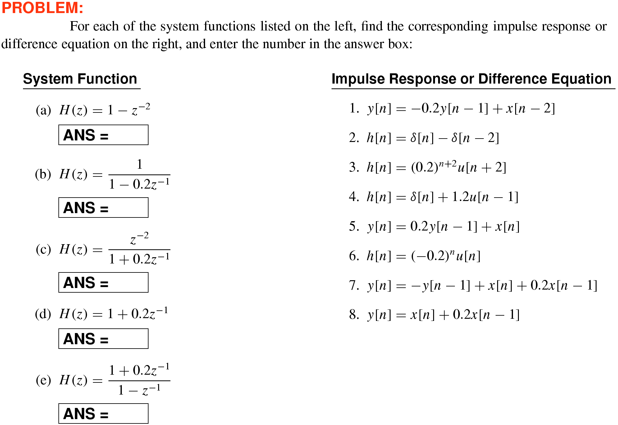
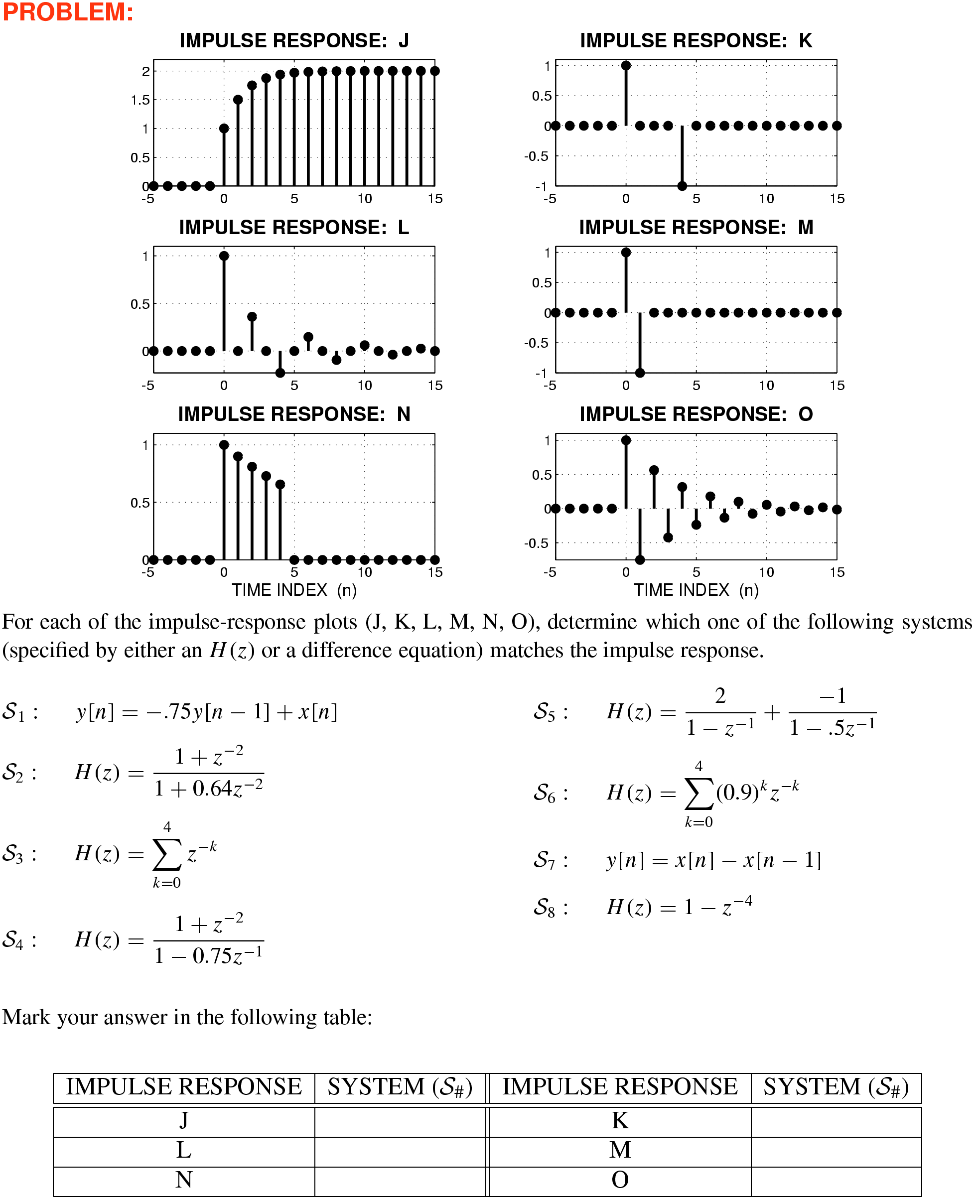
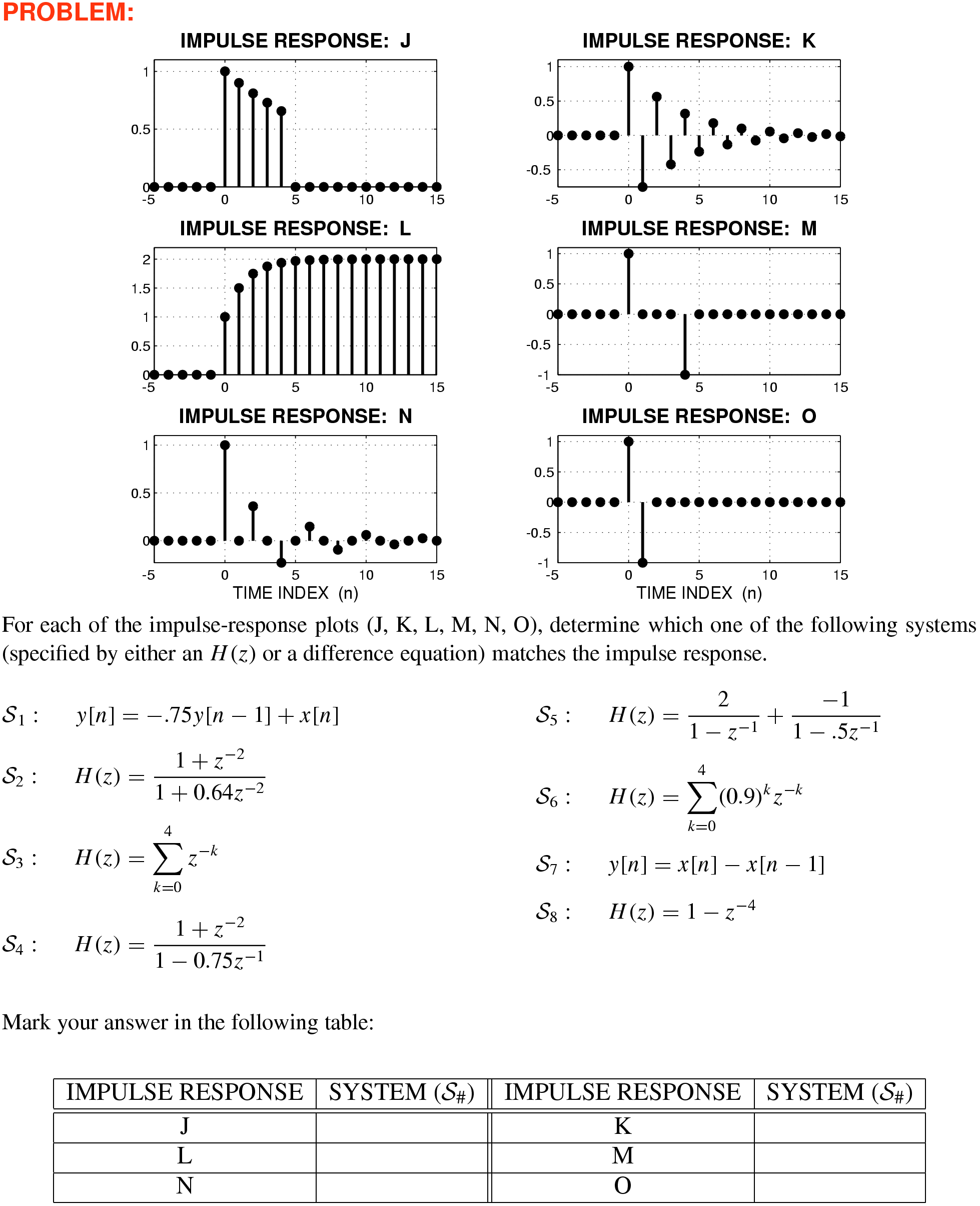
–2 Matching \(H(z)\) with impulse response or difference equation
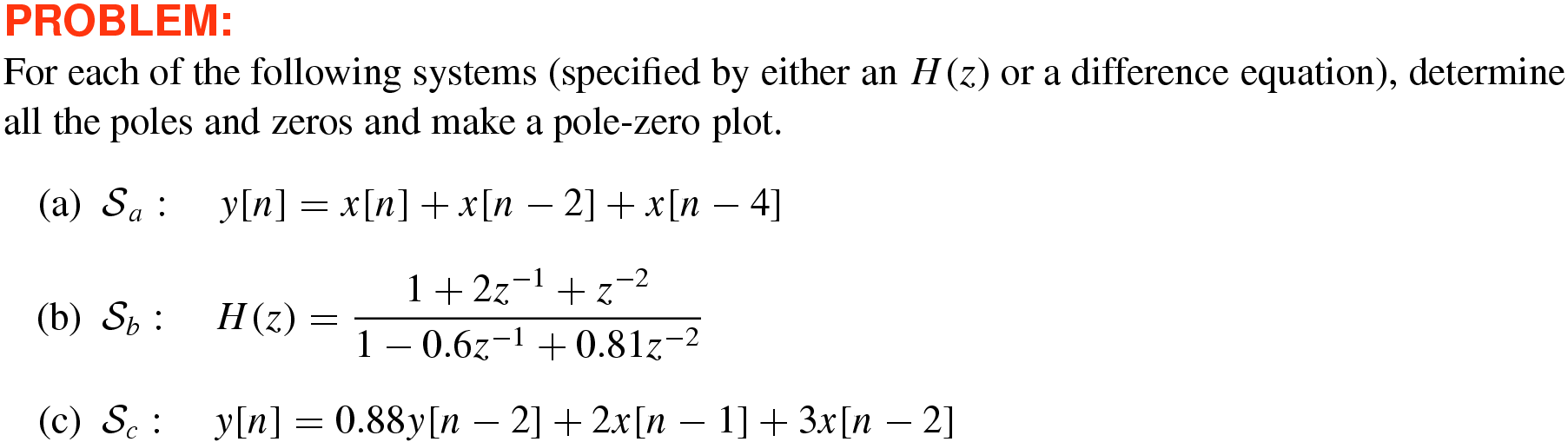
10
–3 Impulse response and \(H(z)\) for cascade
10
–4 Matching \(H(z)\) with impulse response or difference equation
10
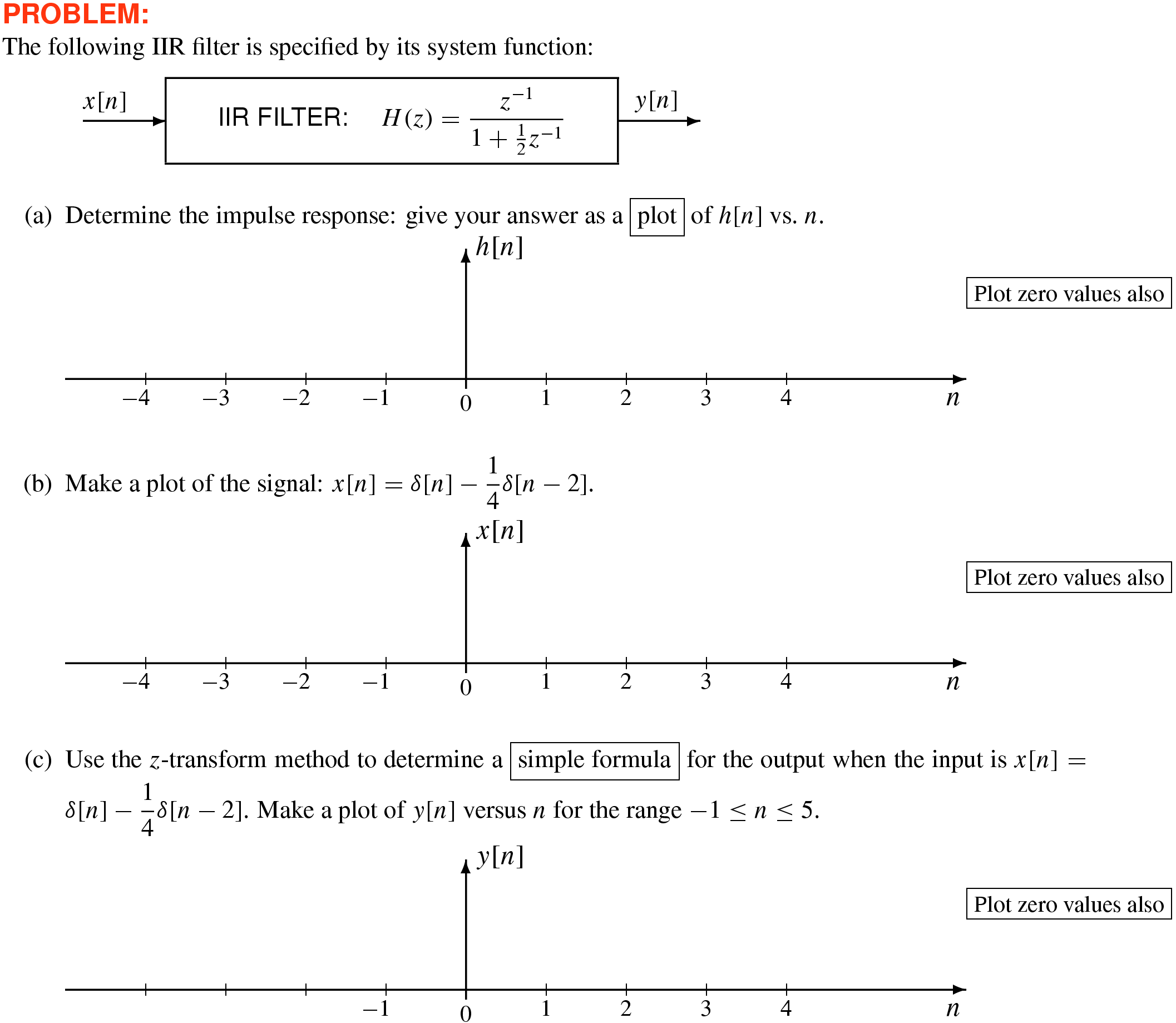
–5 Impulse response and \(H(z)\) for cascade
Solution
10
–6 Matching \(H(z)\) with impulse response or difference equation
Solution
10
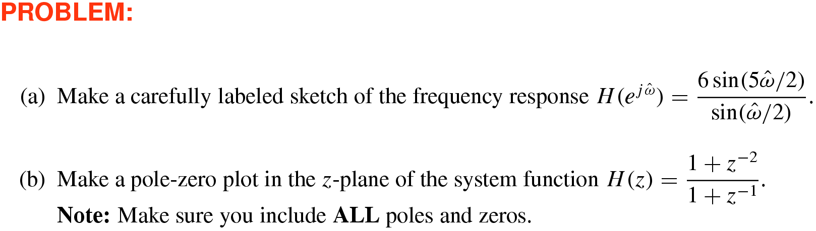
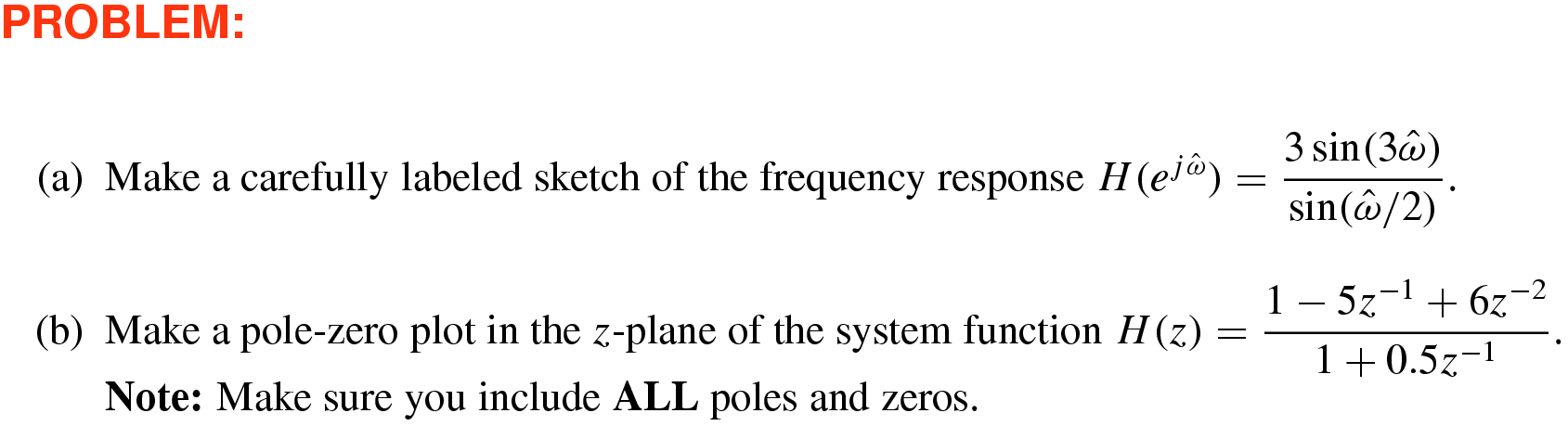
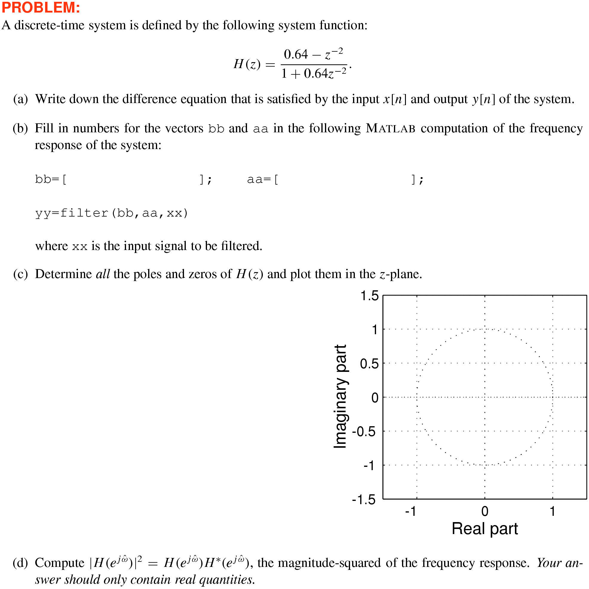
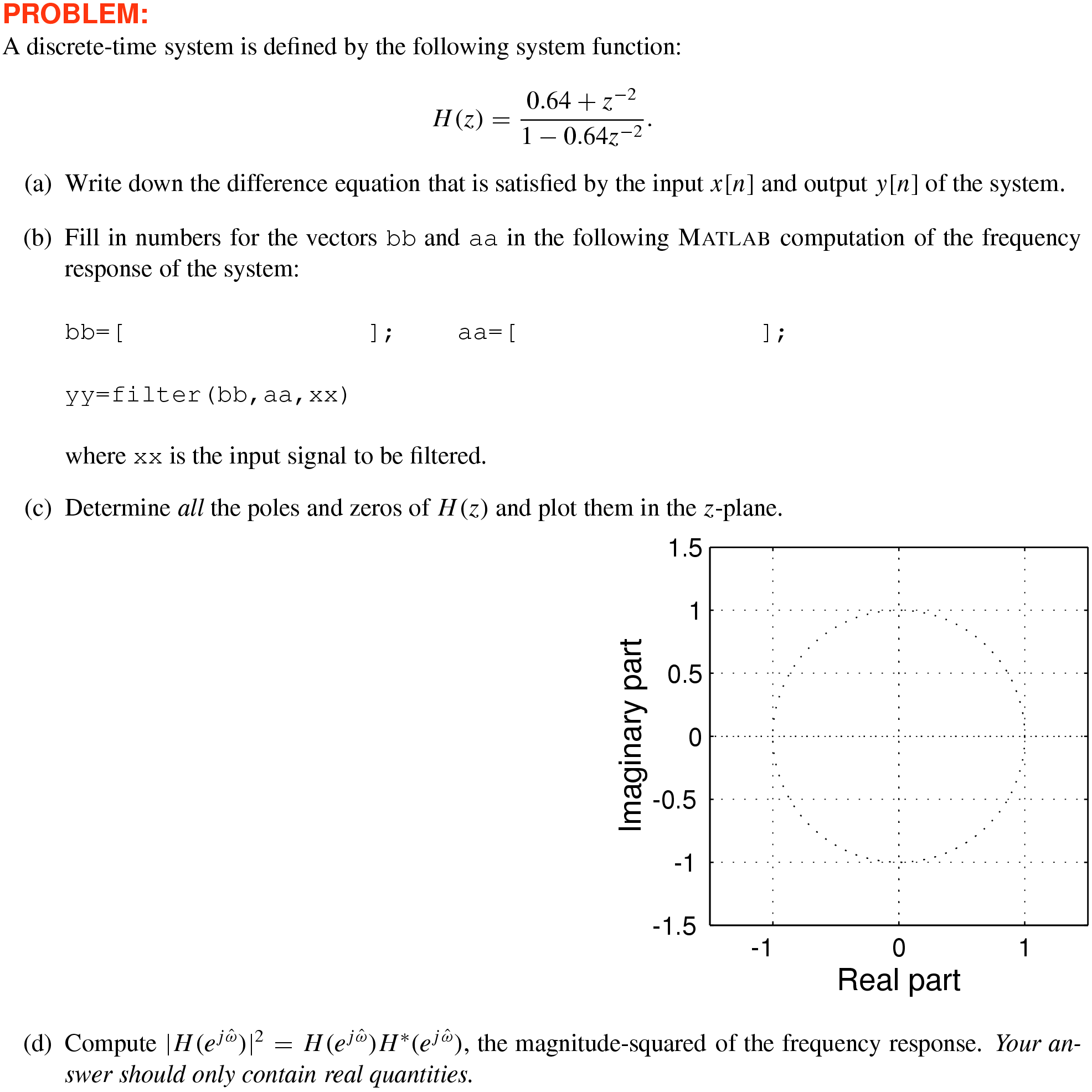
–7 Plot frequency response & pole-zero plot
Solution
10
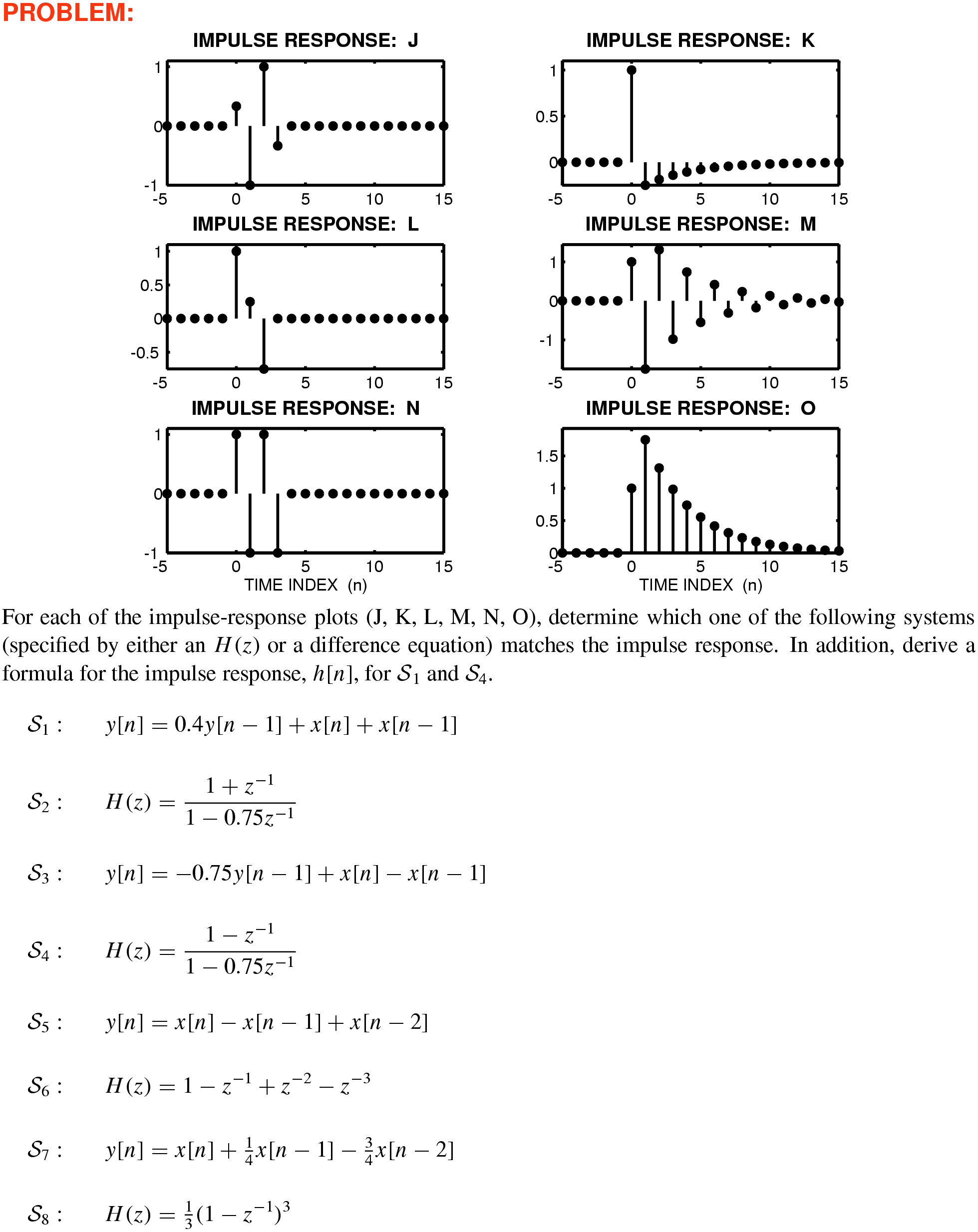
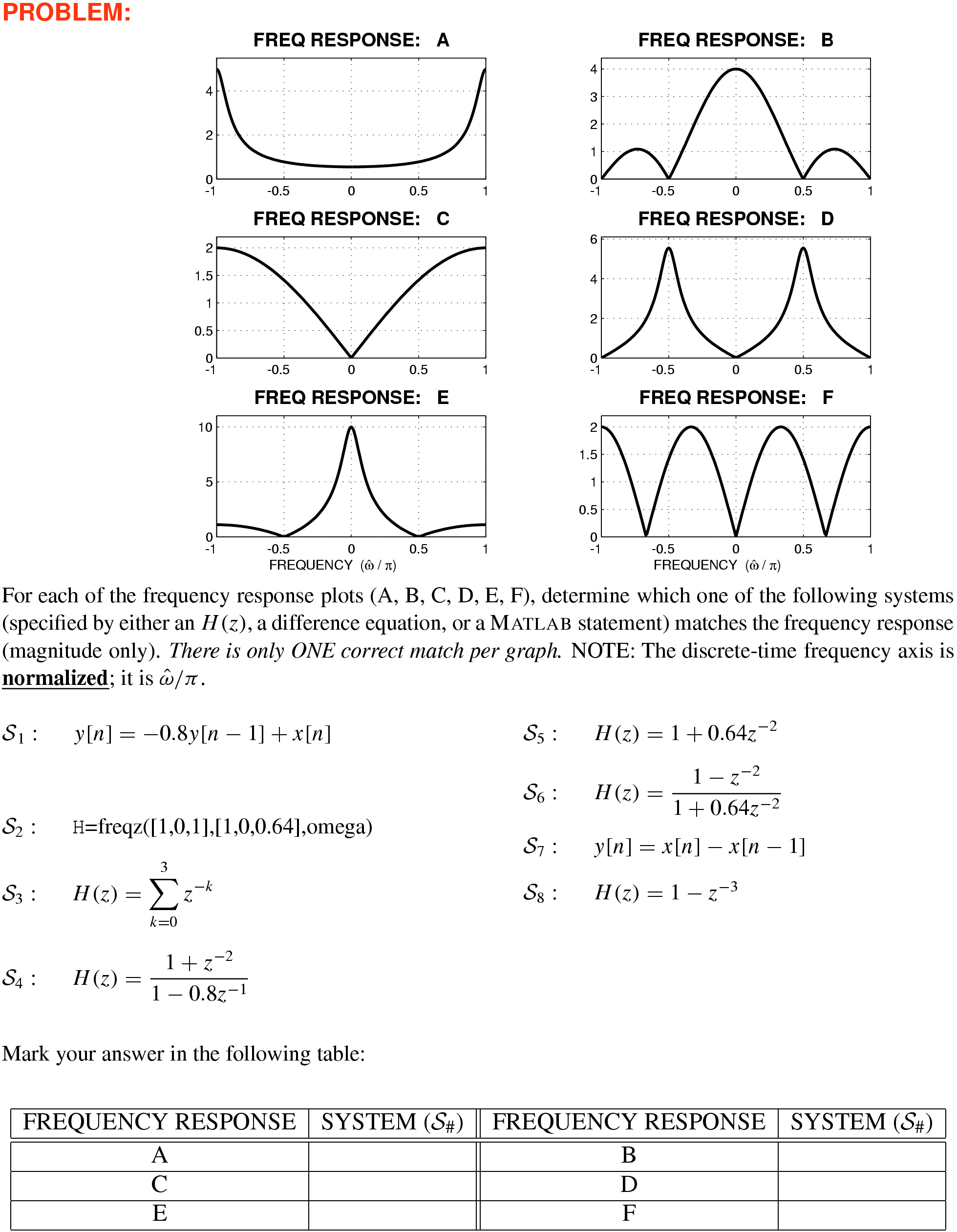
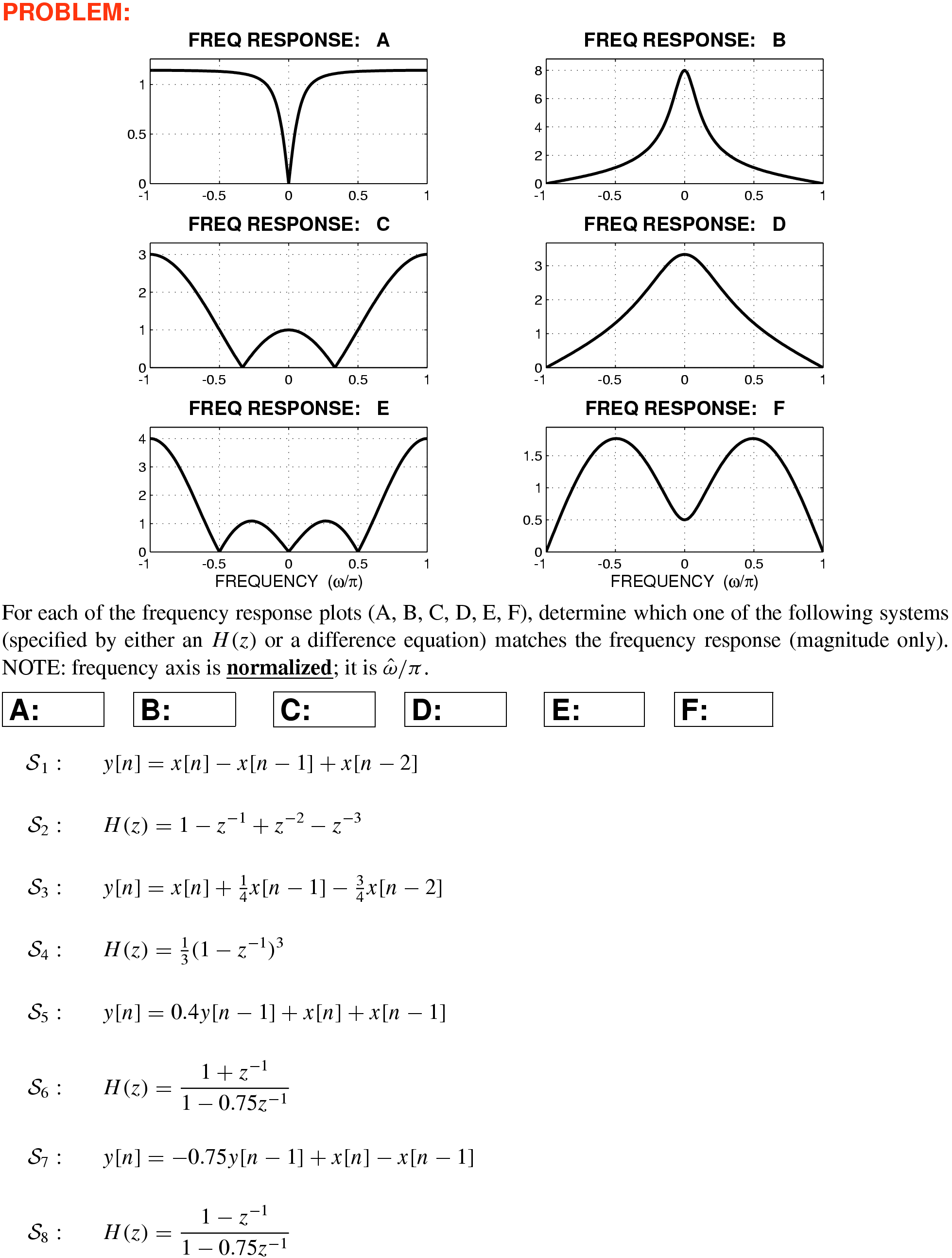
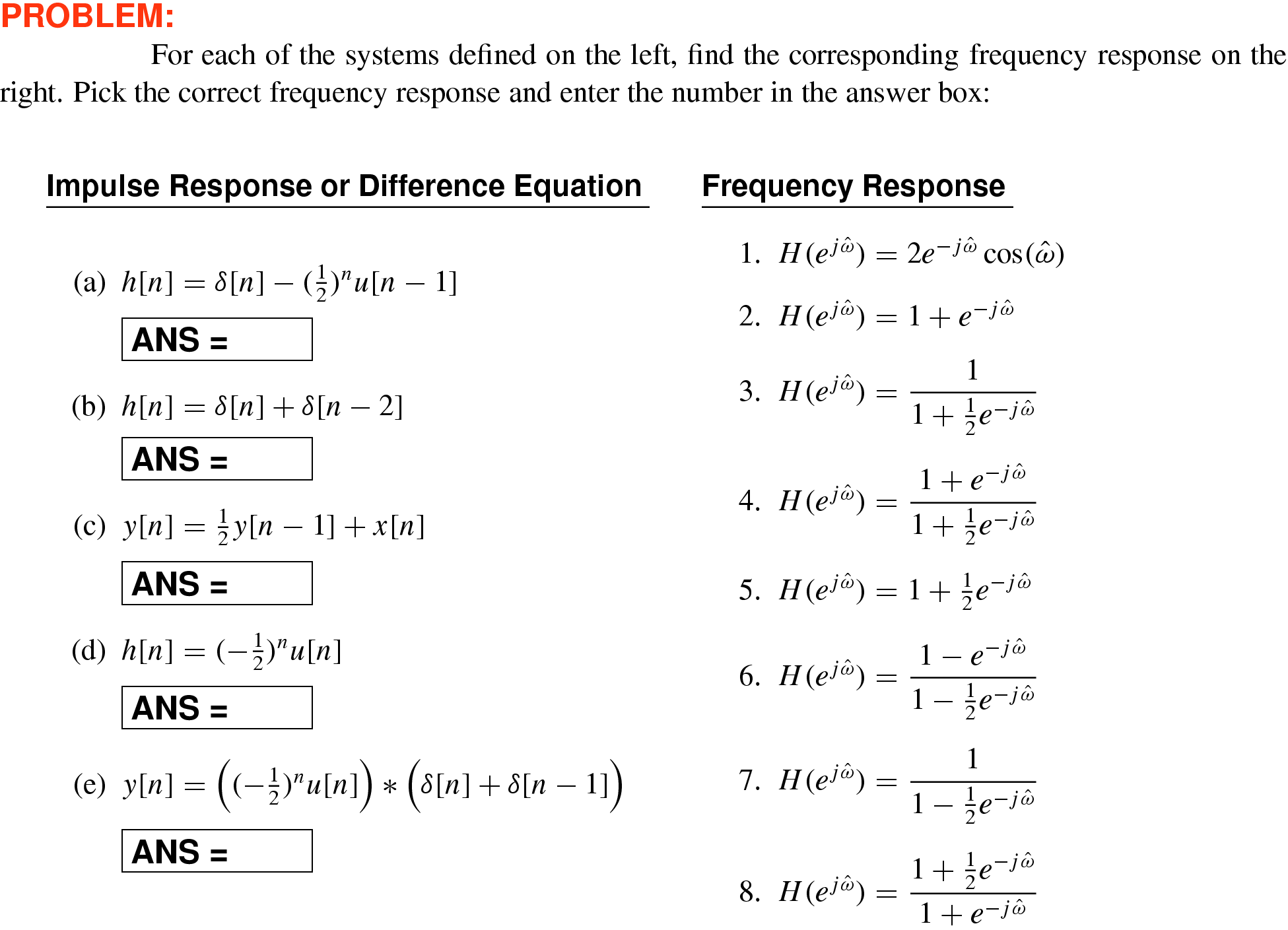
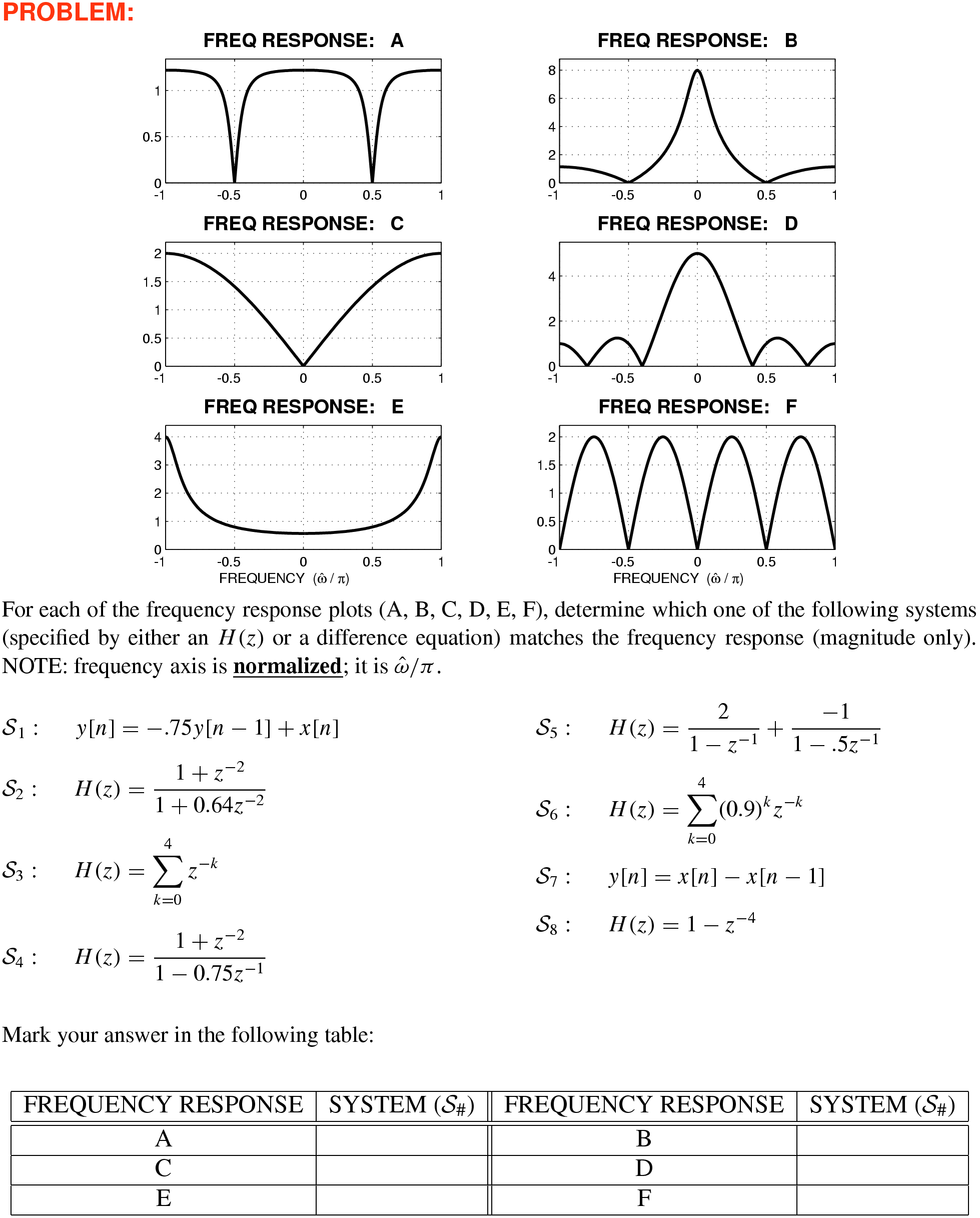
–8 Matching impulse response or difference equation to frequency response
Solution
10
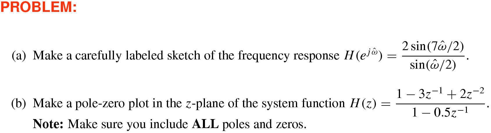
–9 Plot frequency response & pole-zero plot
10
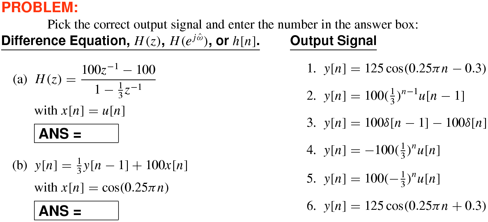
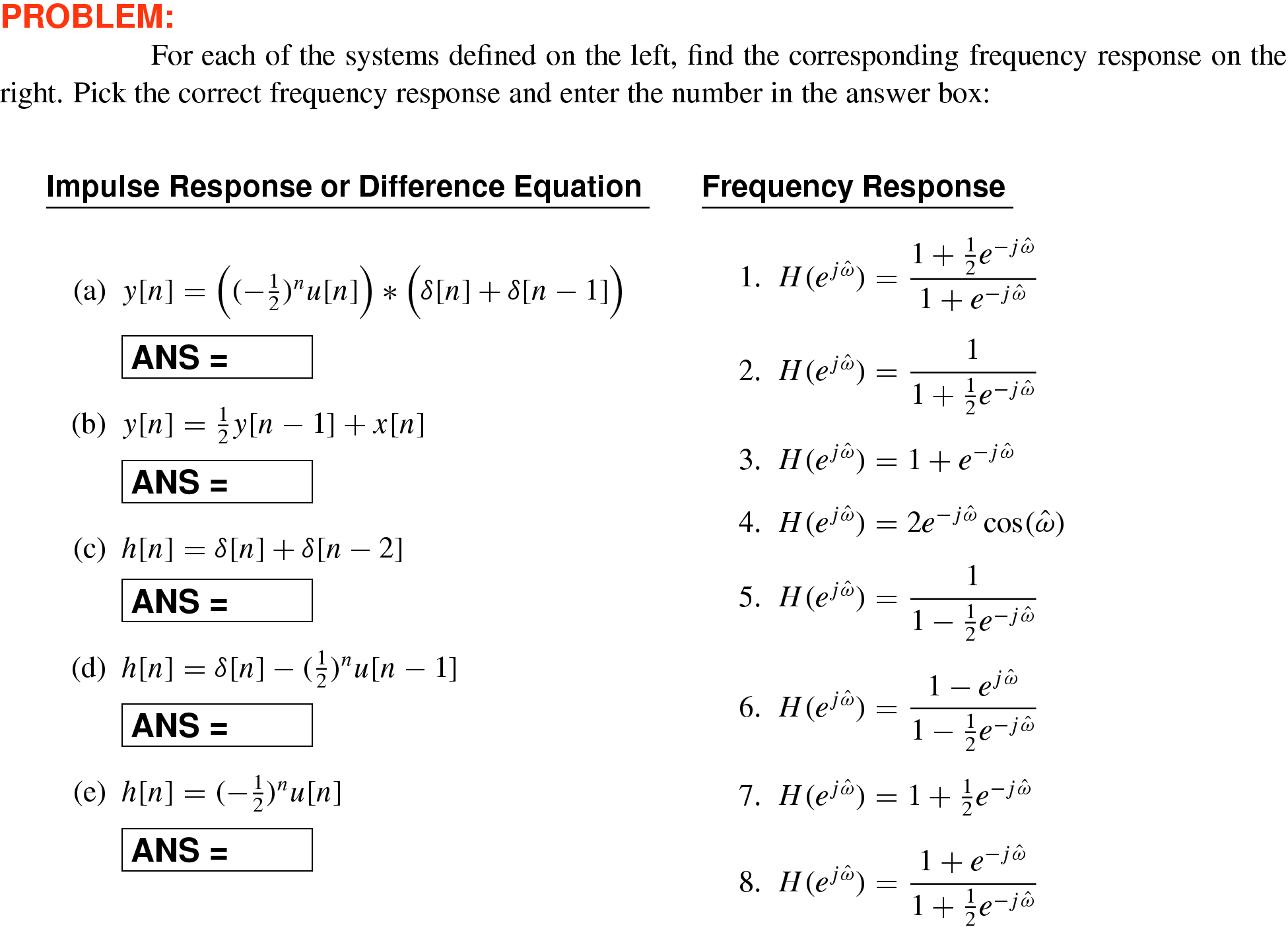
–10 Matching impulse response or difference equation to frequency response
10
–11 Plot frequency response & pole-zero plot
10
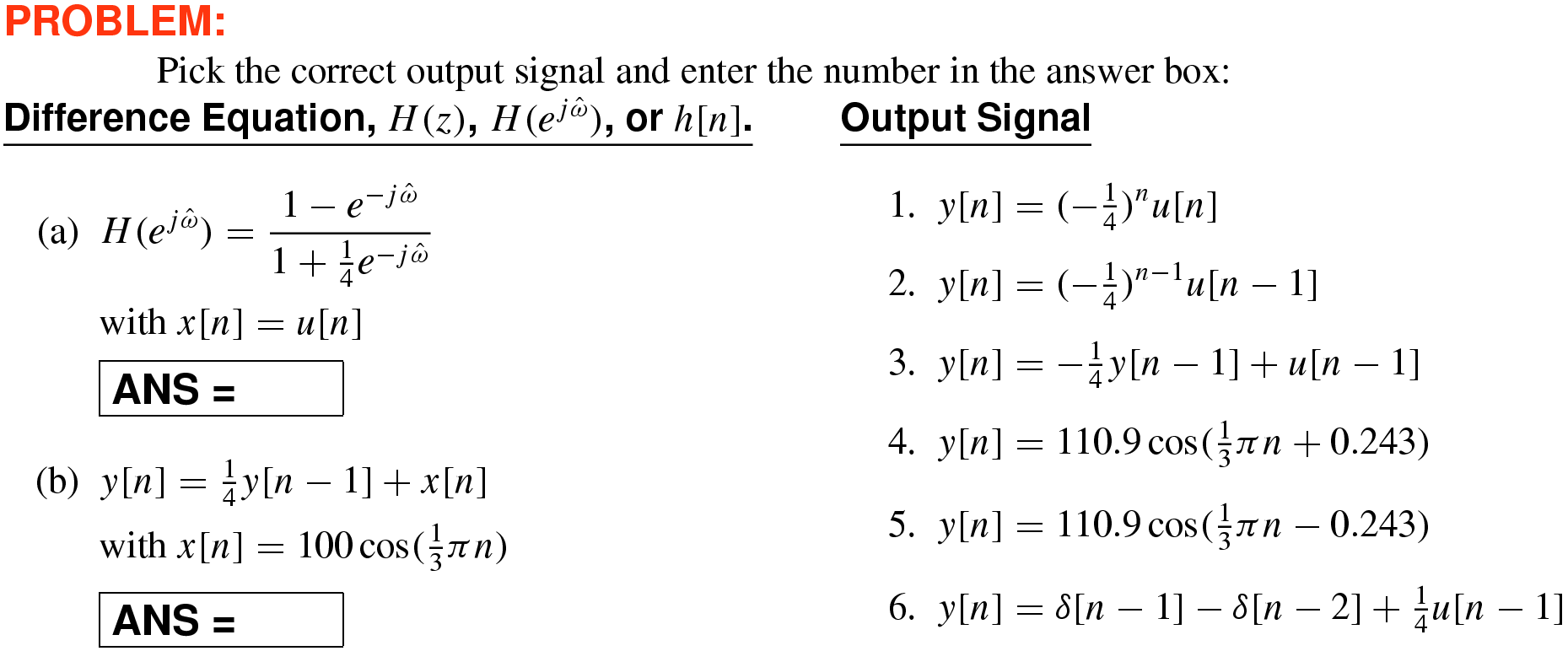
–12 Matching impulse response or difference equation to frequency response
10
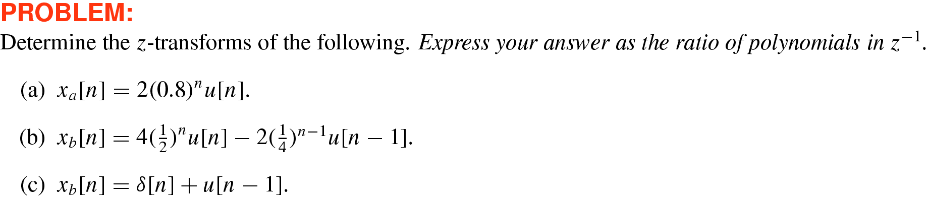
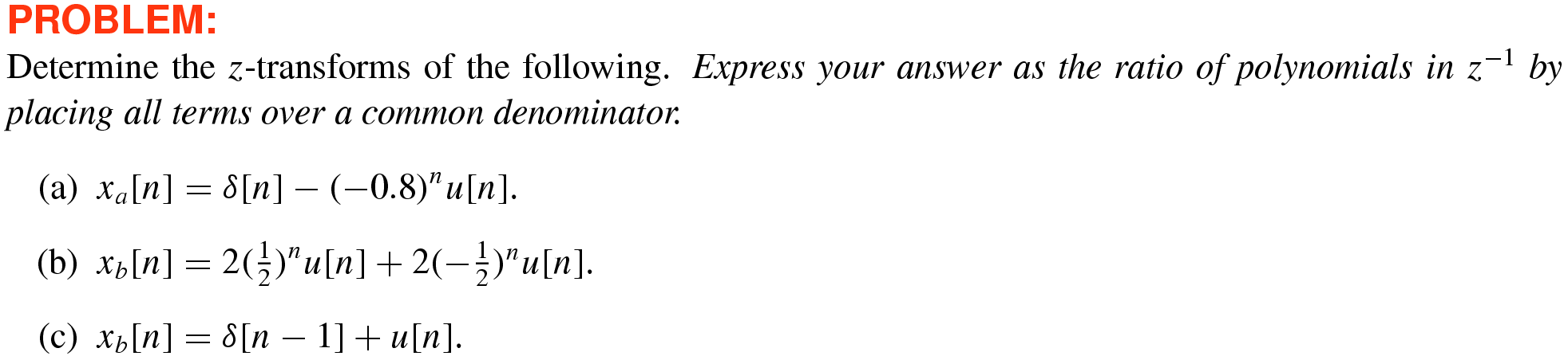
–13 Various \(z\mbox{-}\)transforms
Solution
10
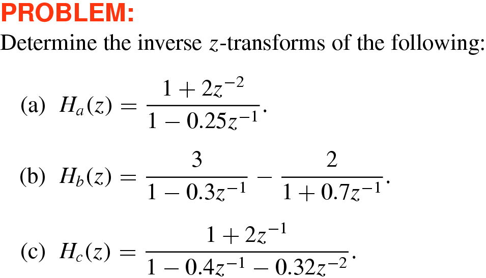
–14 Various inverse \(z\mbox{-}\)transforms
Solution
10
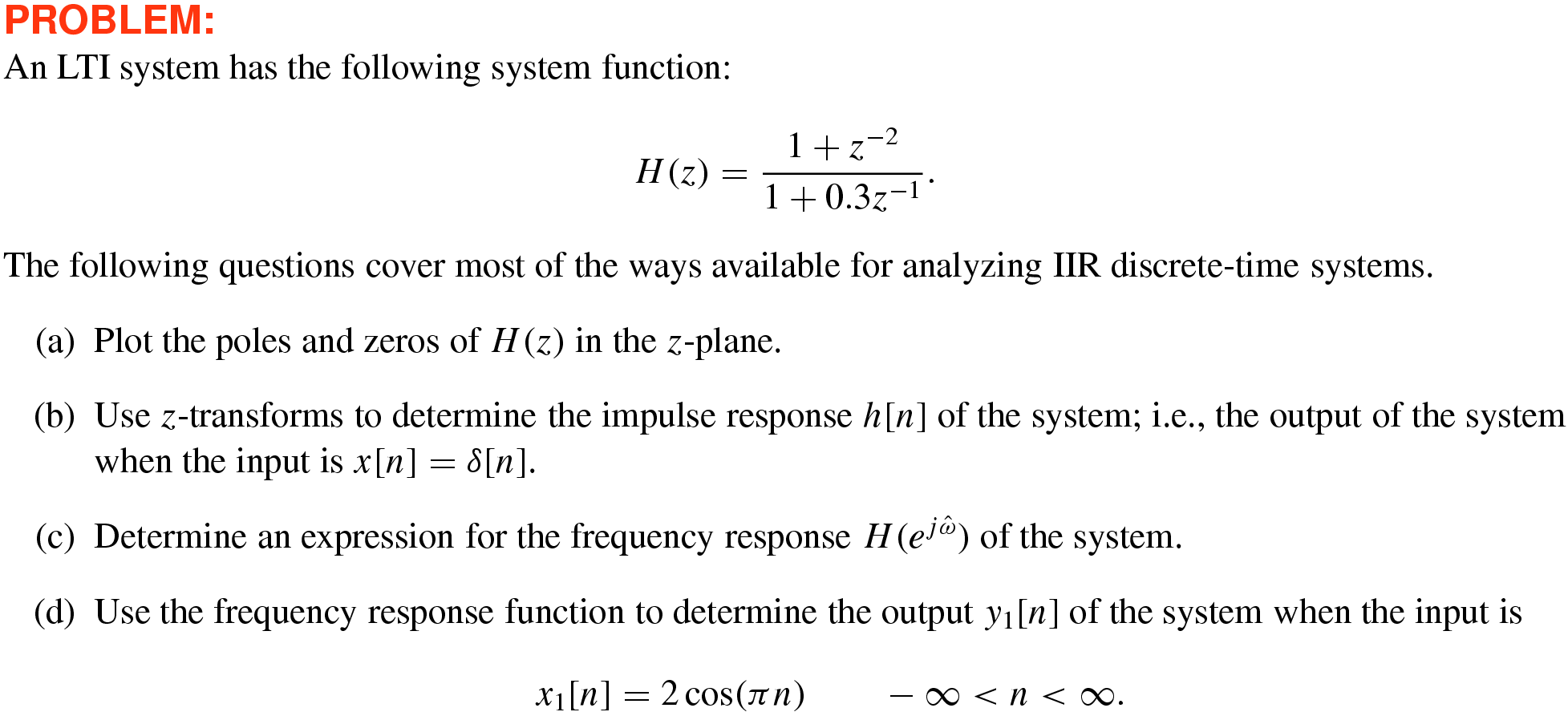
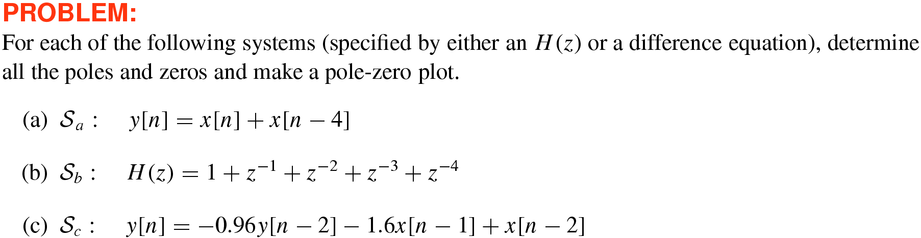
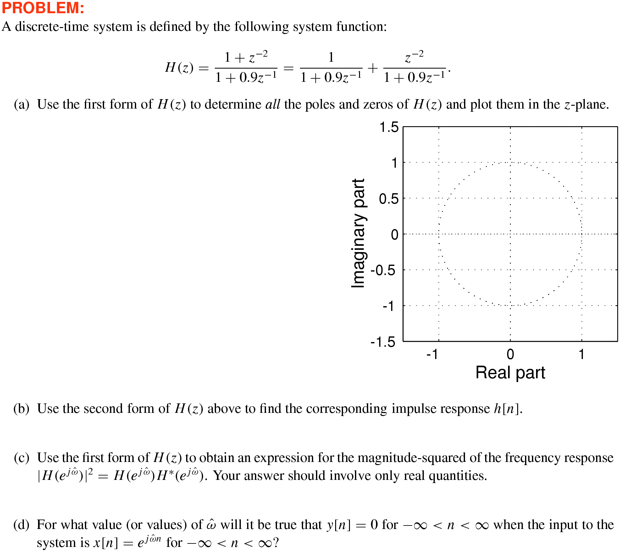
–15 Three-domain analysis for IIR system given \(H(z)\)
Solution
10
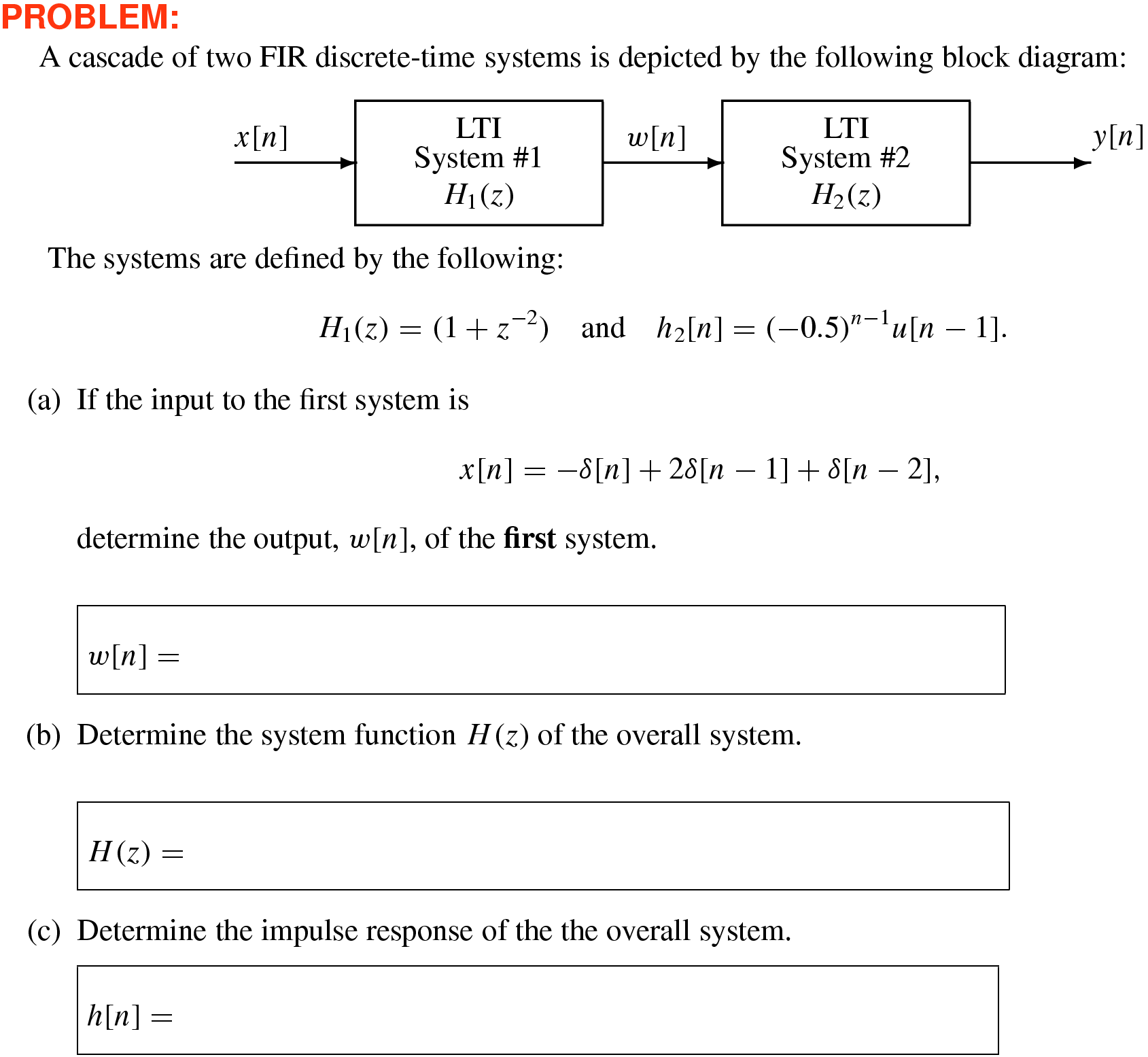
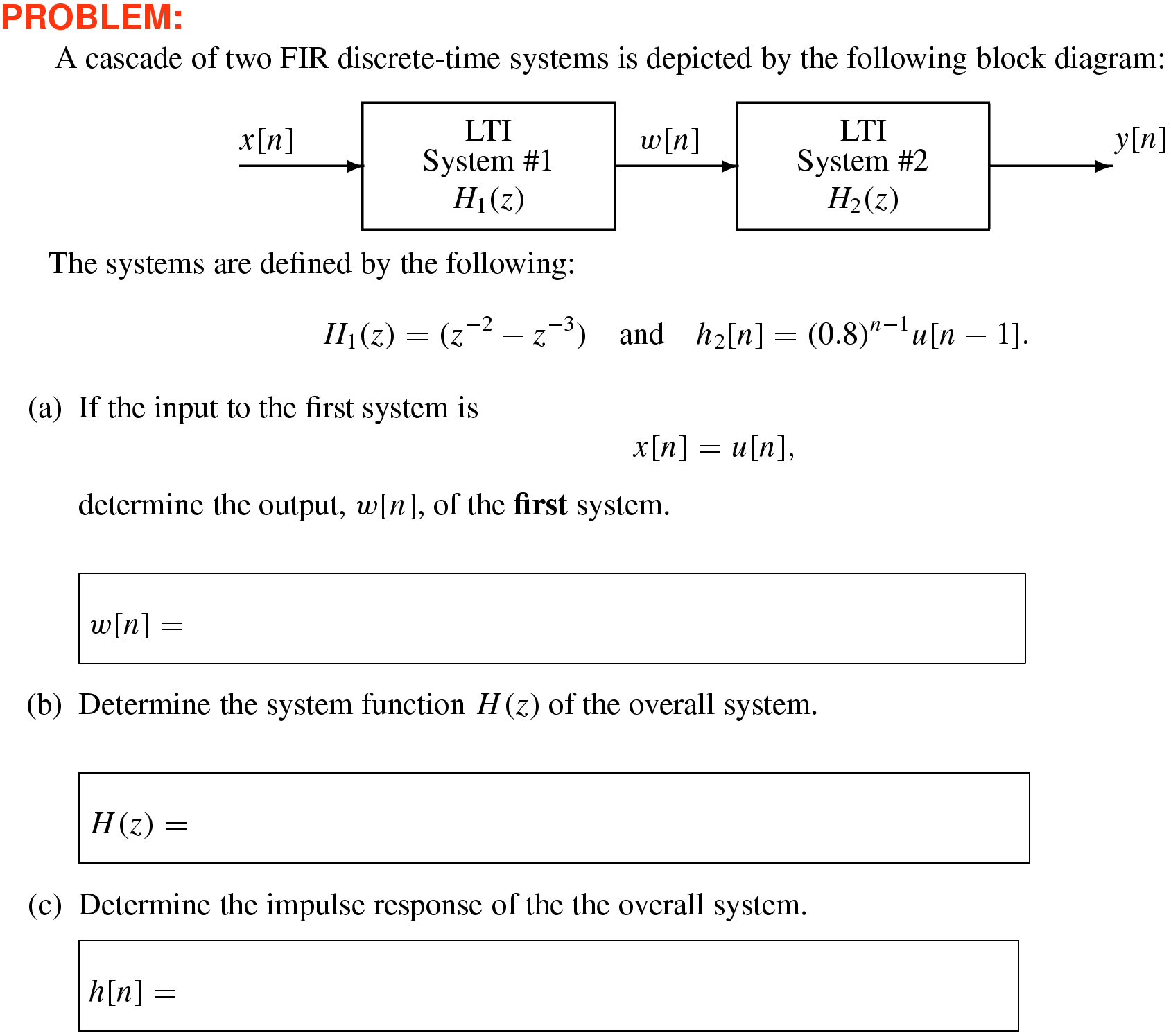
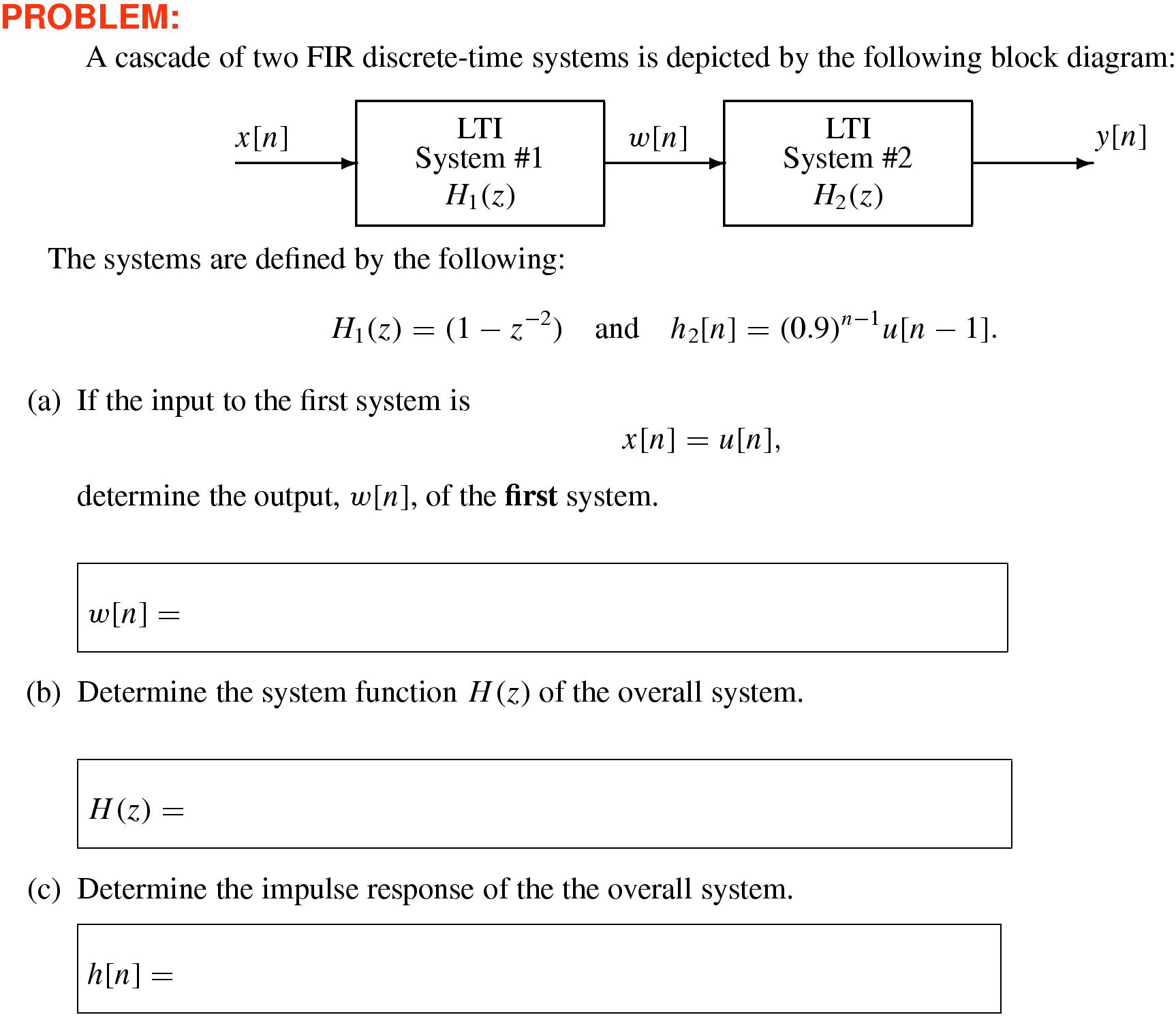
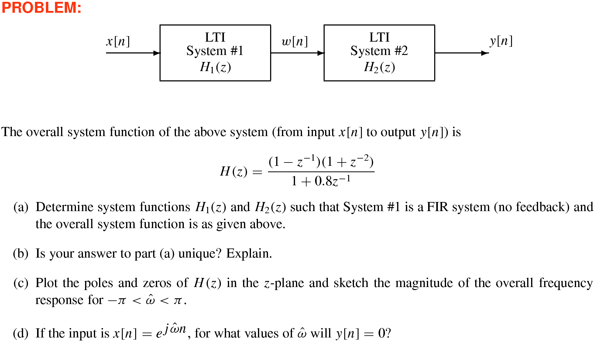
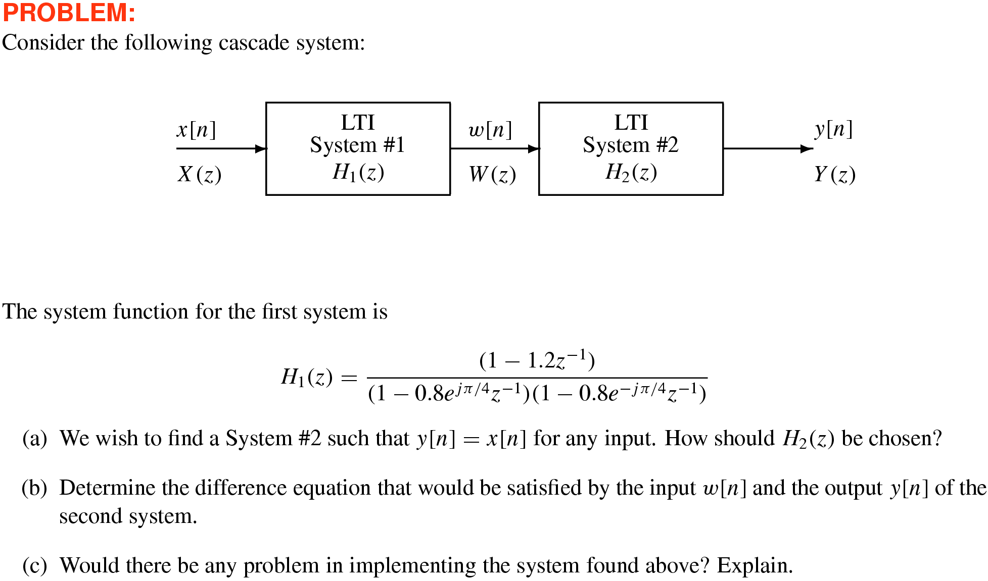
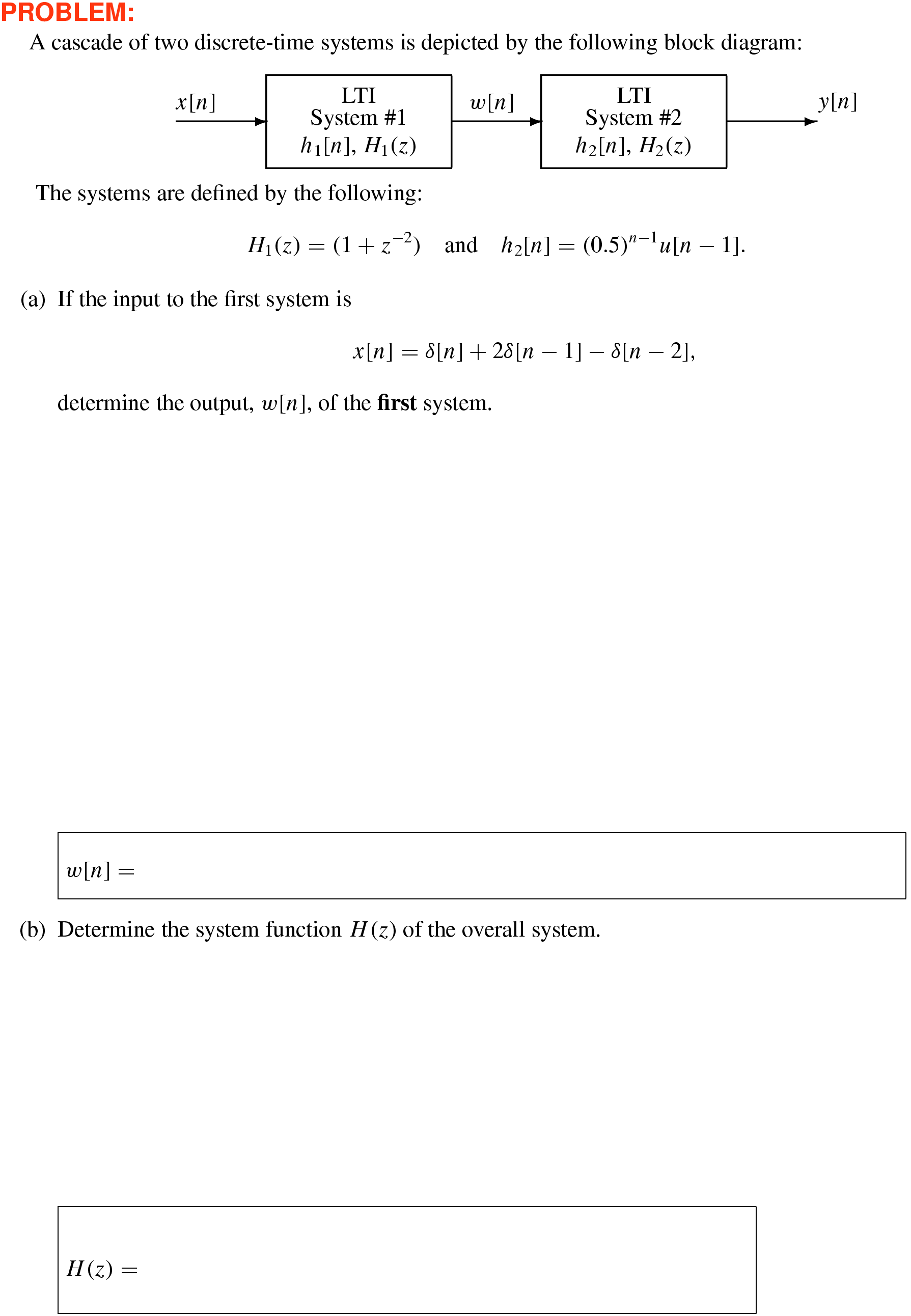
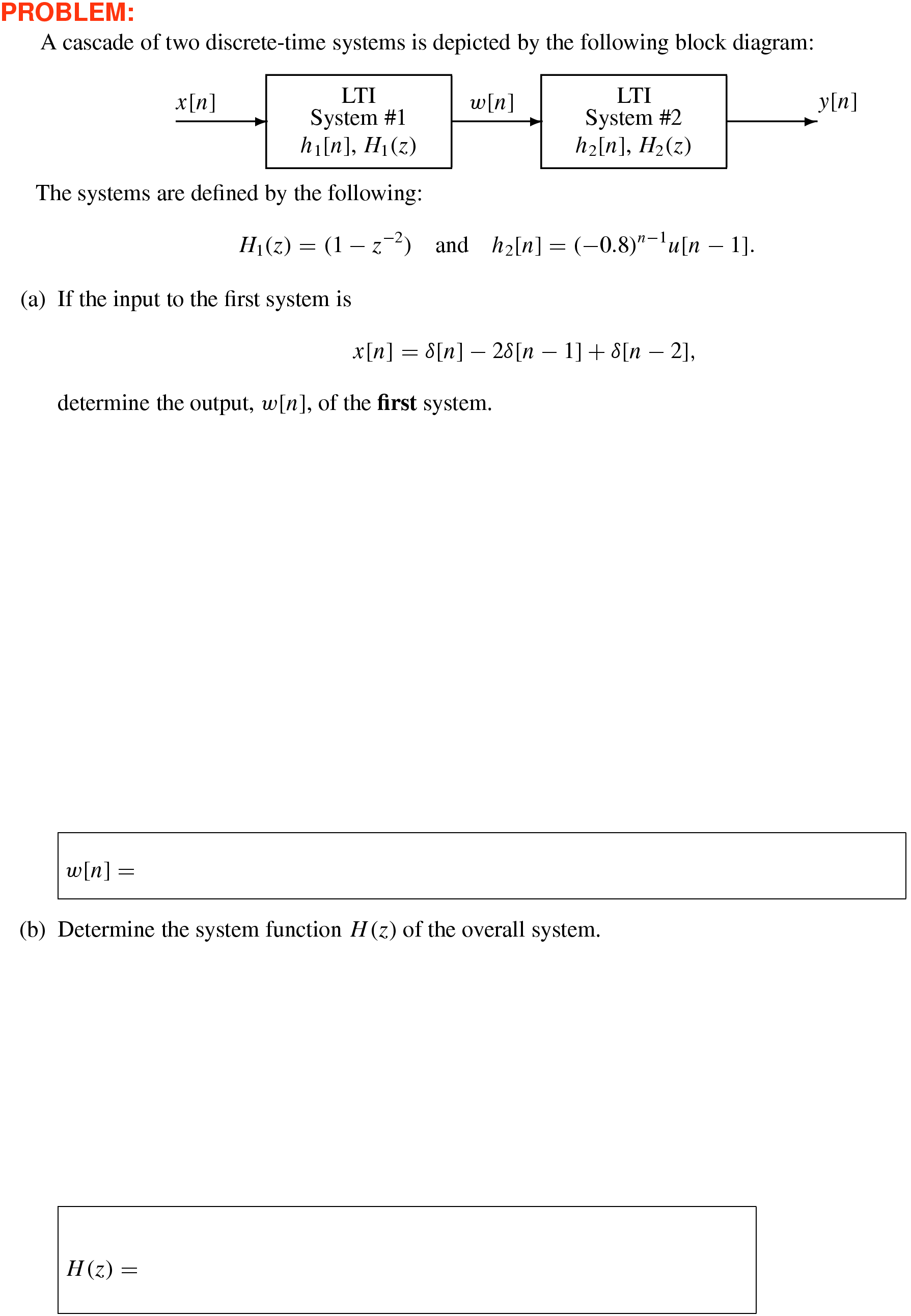
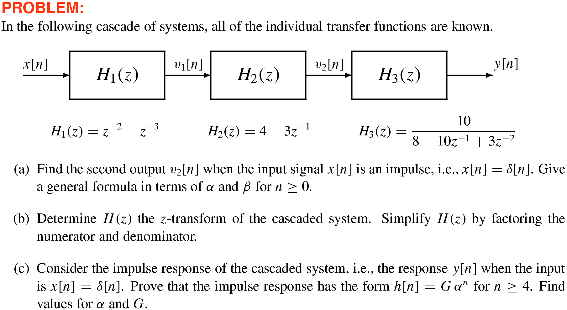
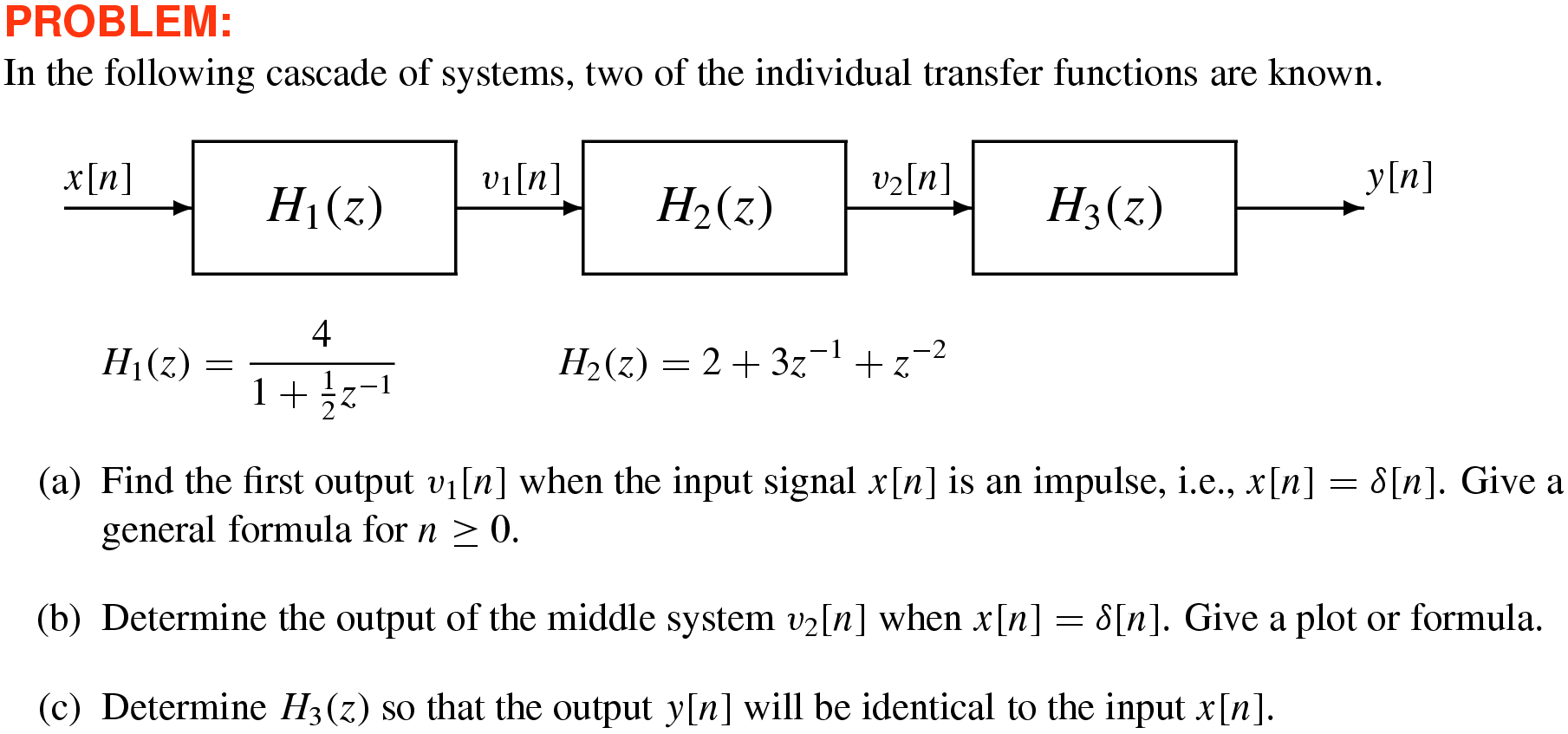
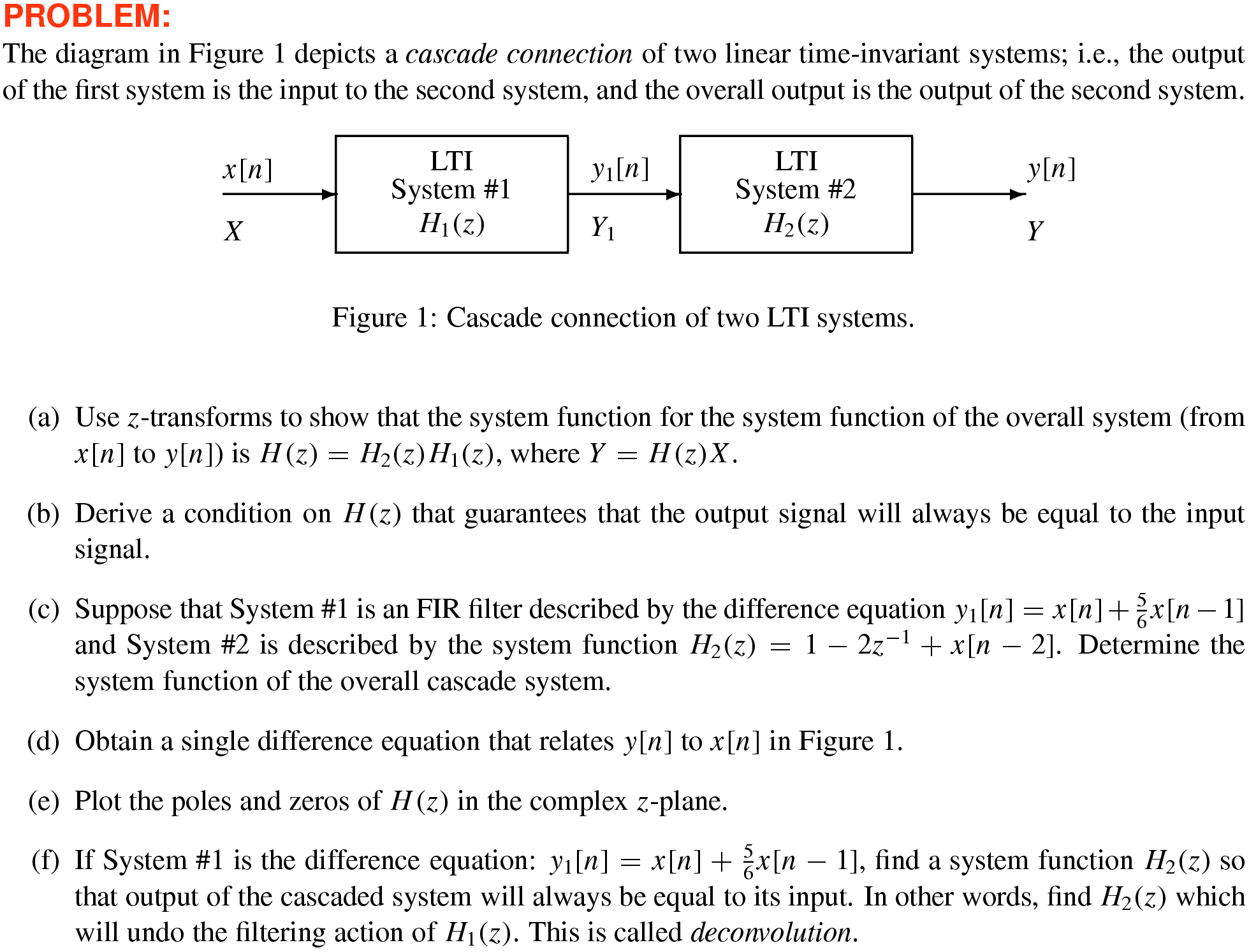
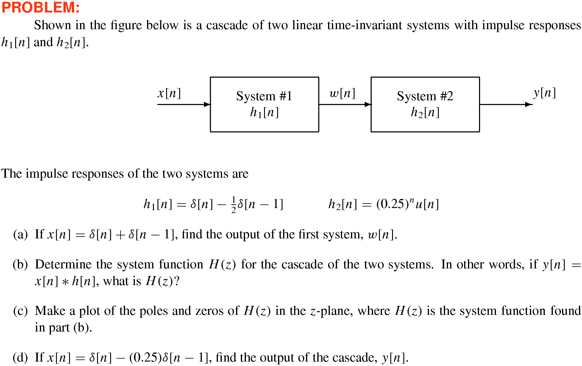
–16 Cascade of Two Discrete-Time Systems ♦ Find \(H(z)\)
Solution
10
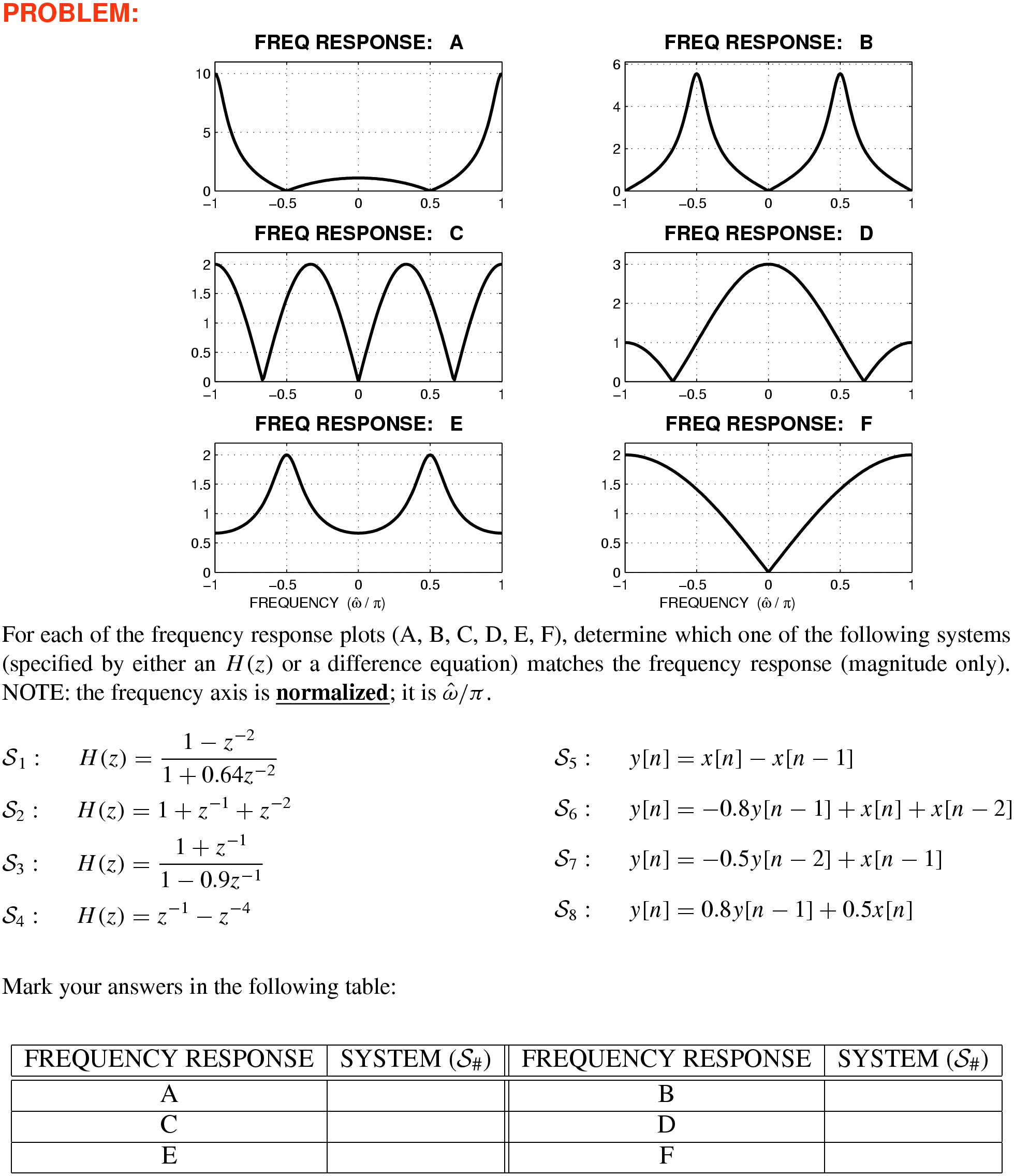
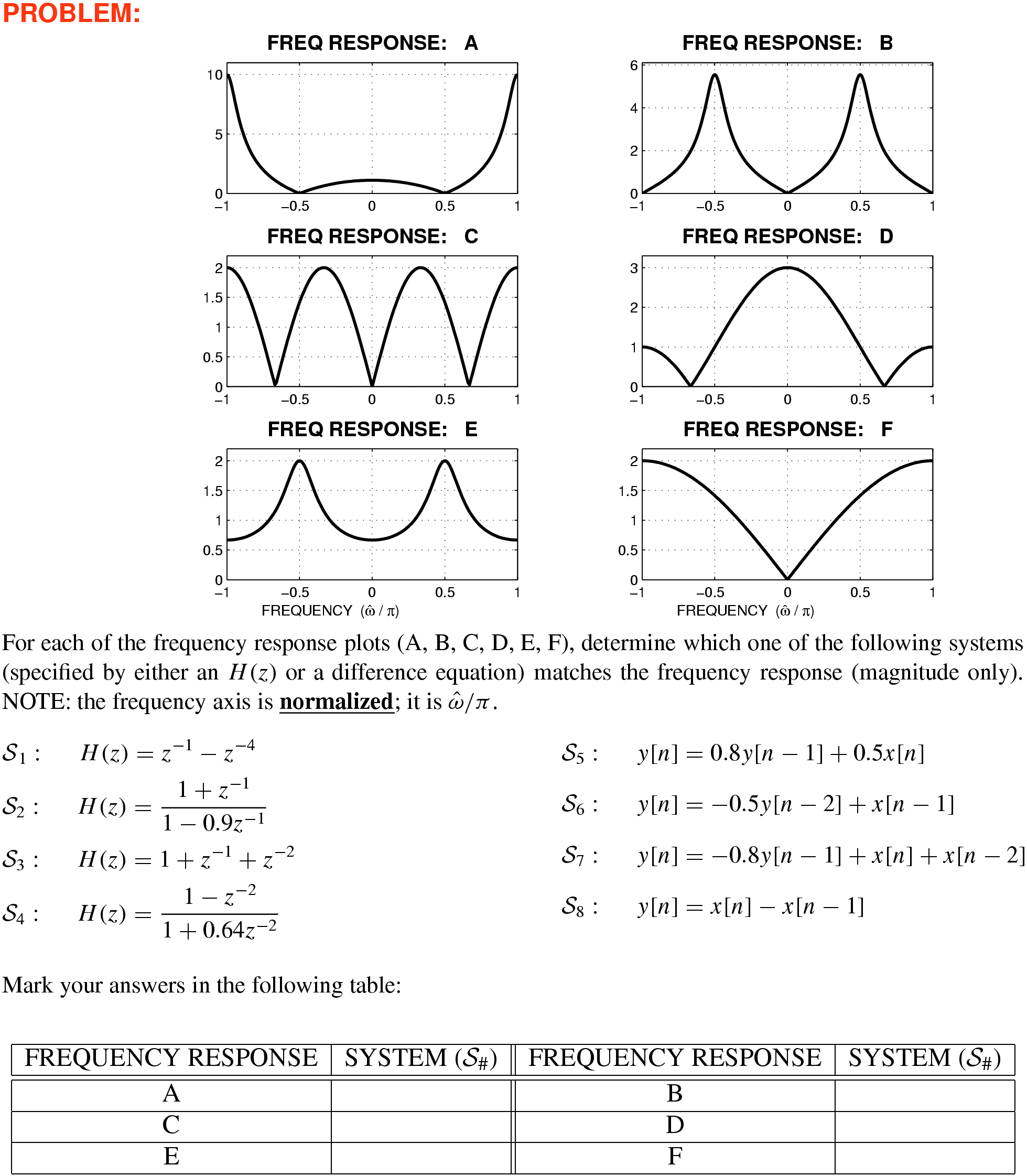
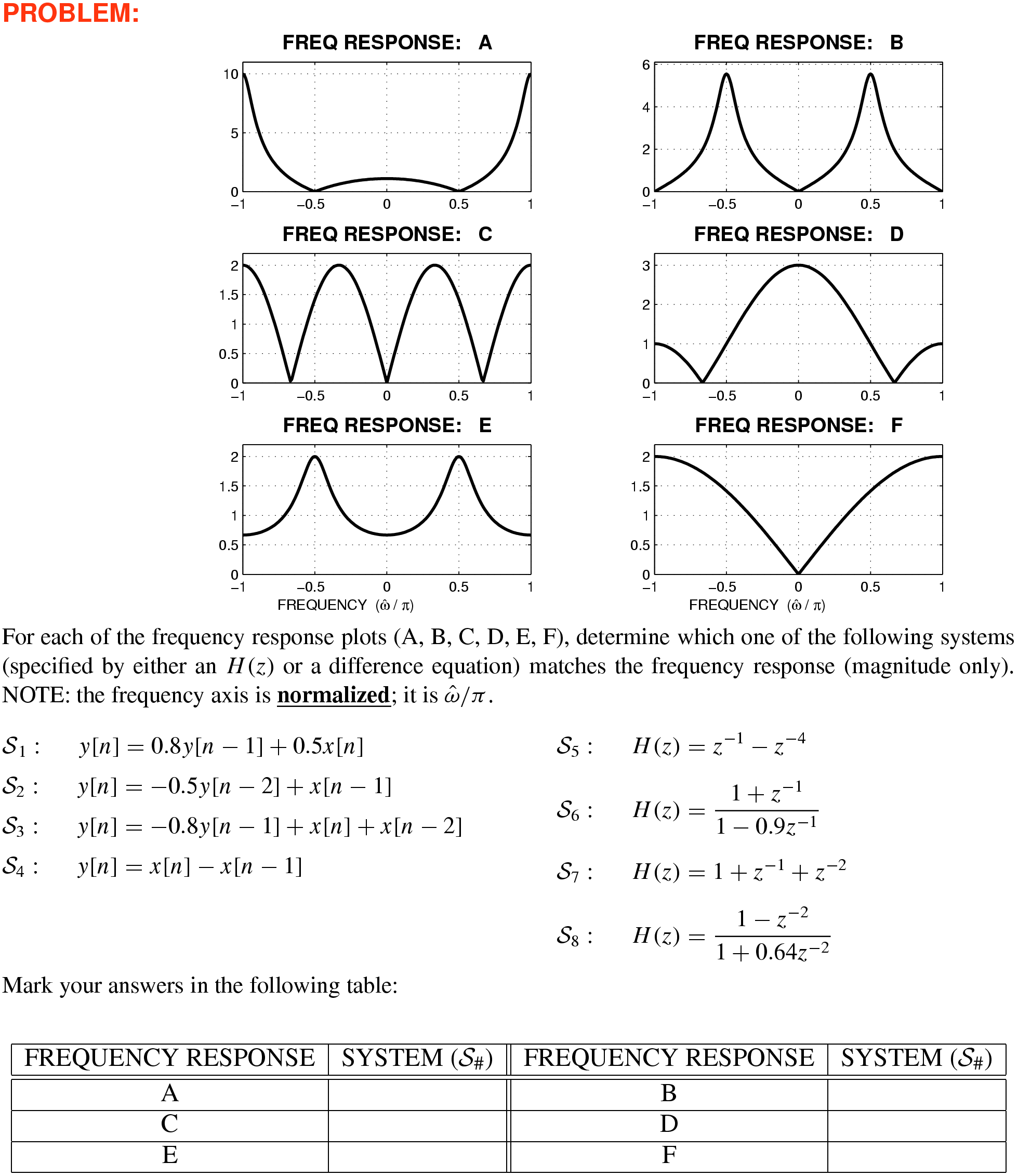
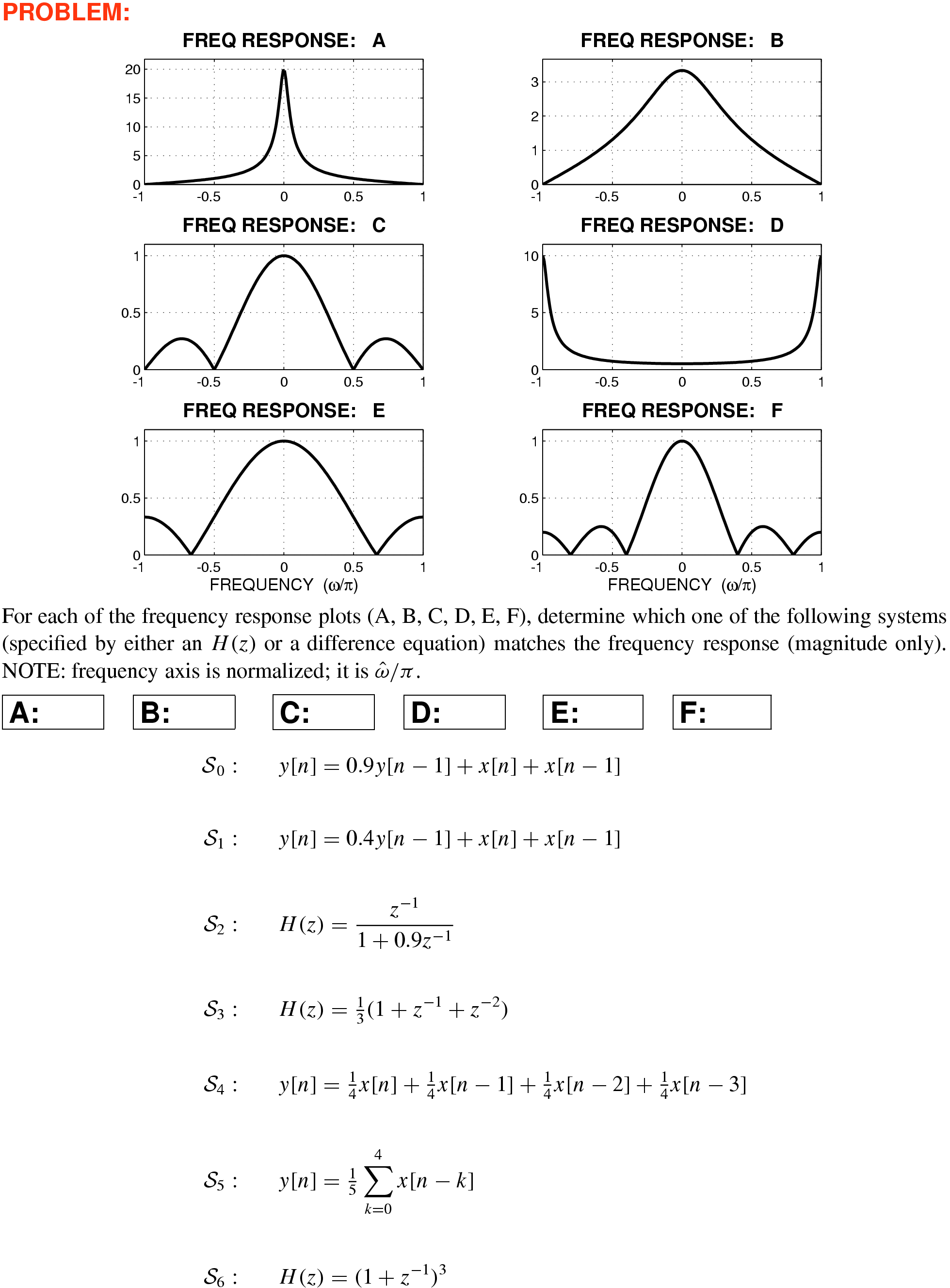
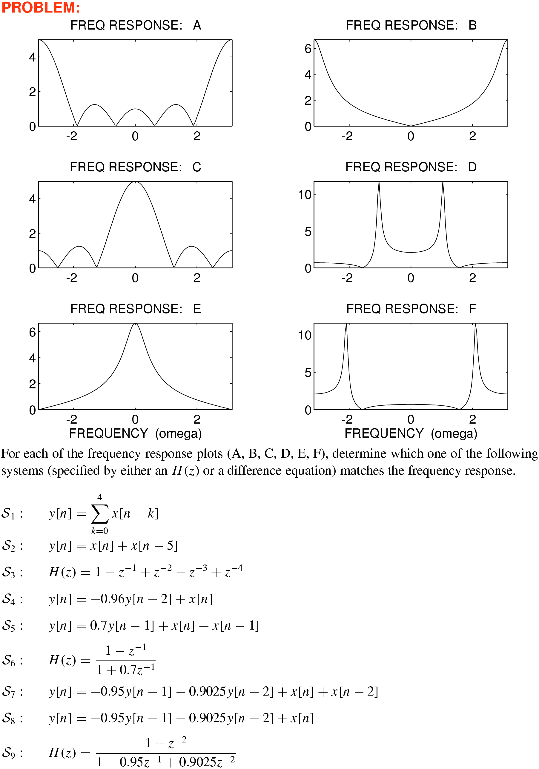
–17 Match the Frequency Response with \(H(z)\) or the Difference Equation
Solution
10
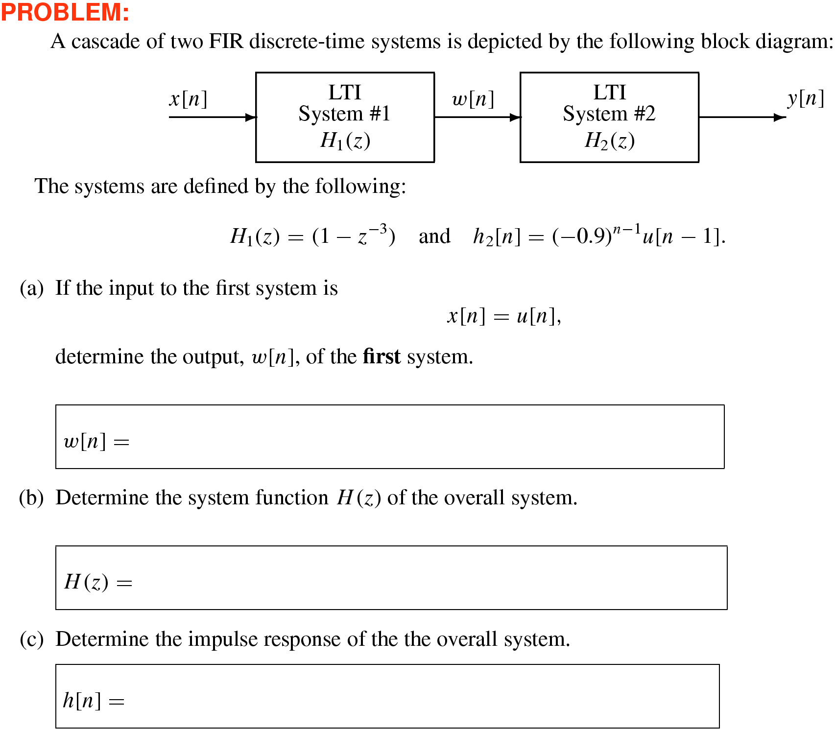
–18 Cascade of Two Discrete-Time Systems ♦ Find \(H(z)\)
Solution
10
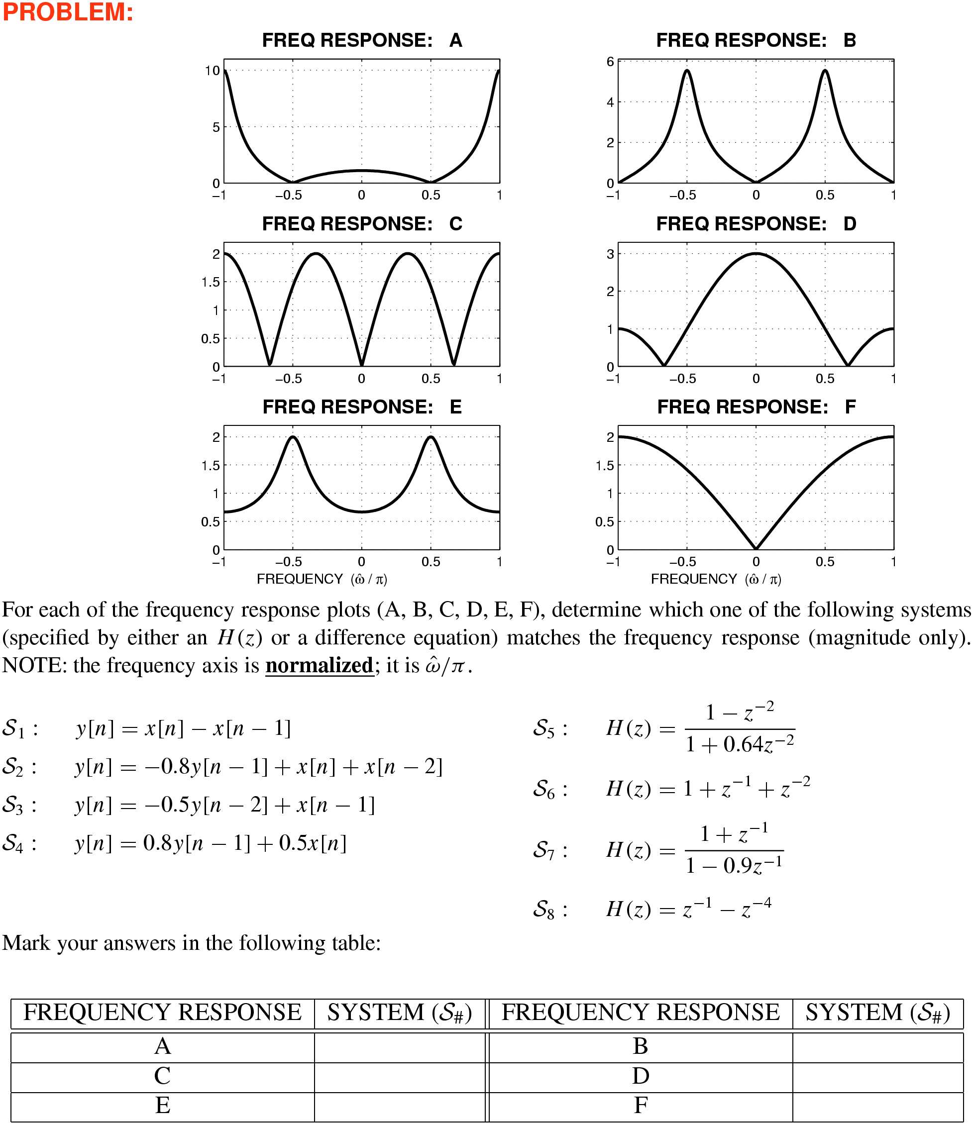
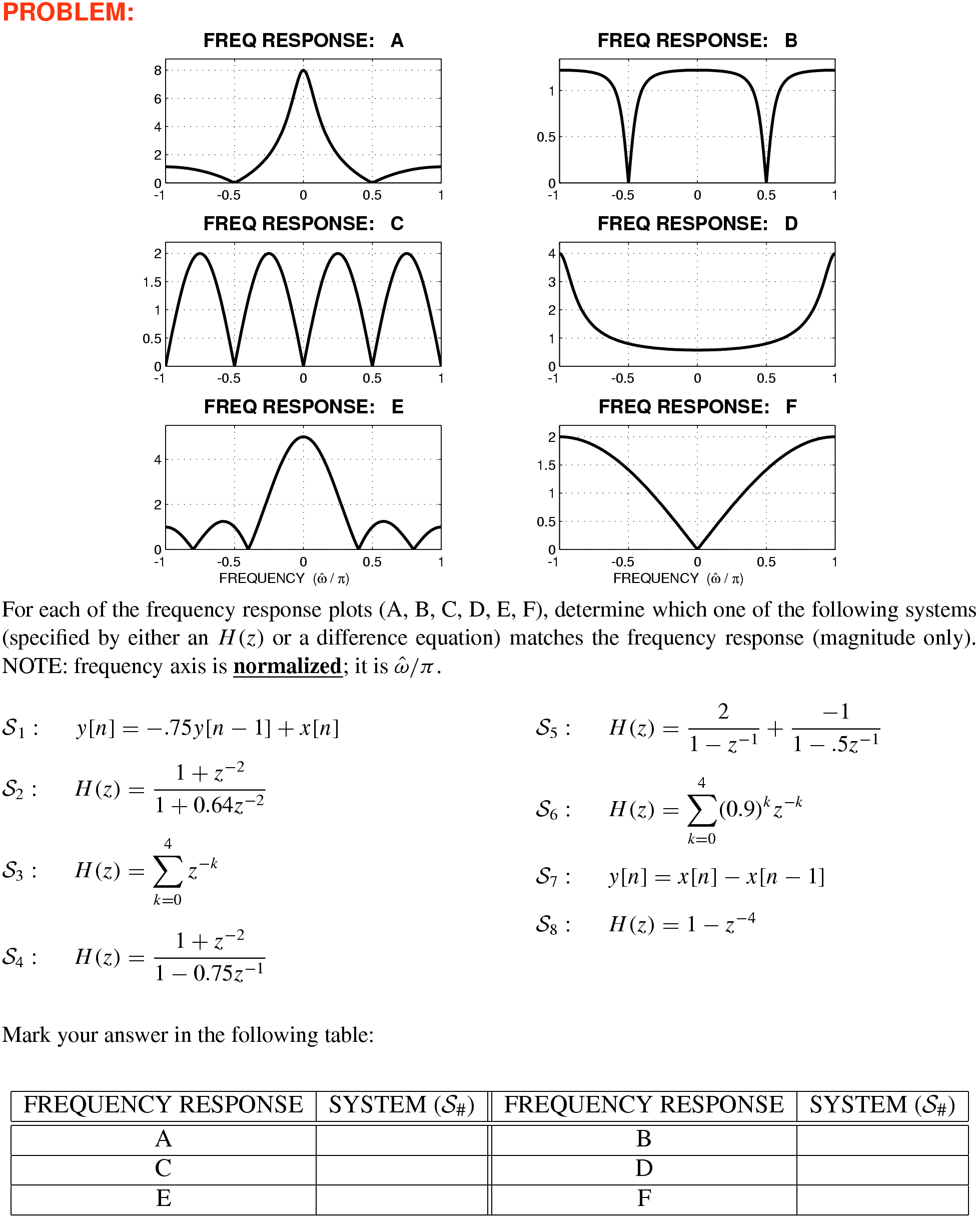
–19 Match the Frequency Response with \(H(z)\) or the Difference Equation
Solution
10
–20 Cascade of Two Discrete-Time Systems ♦ Find \(H(z)\)
Solution
10
–21 Match the Frequency Response with \(H(z)\) or the Difference Equation
Solution
10
–22 Cascade of Two Discrete-Time Systems ♦ Find \(H(z)\)
Solution
10
–23 Match the Frequency Response with \(H(z)\) or the Difference Equation
Solution
10
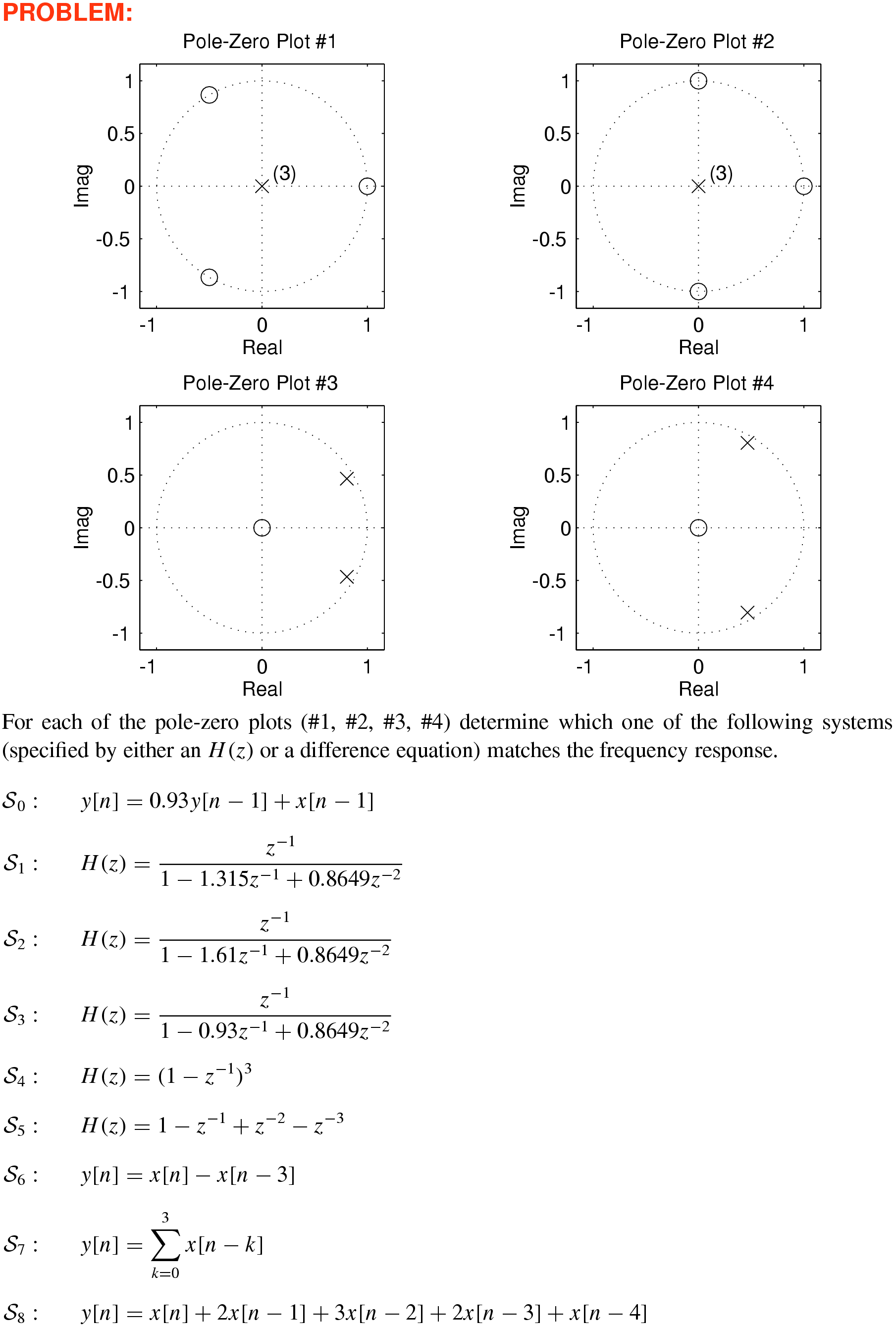
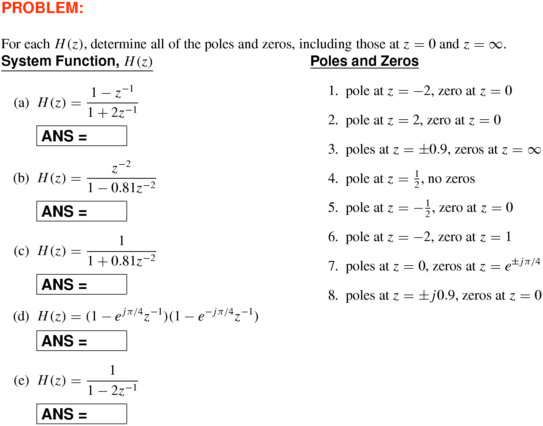
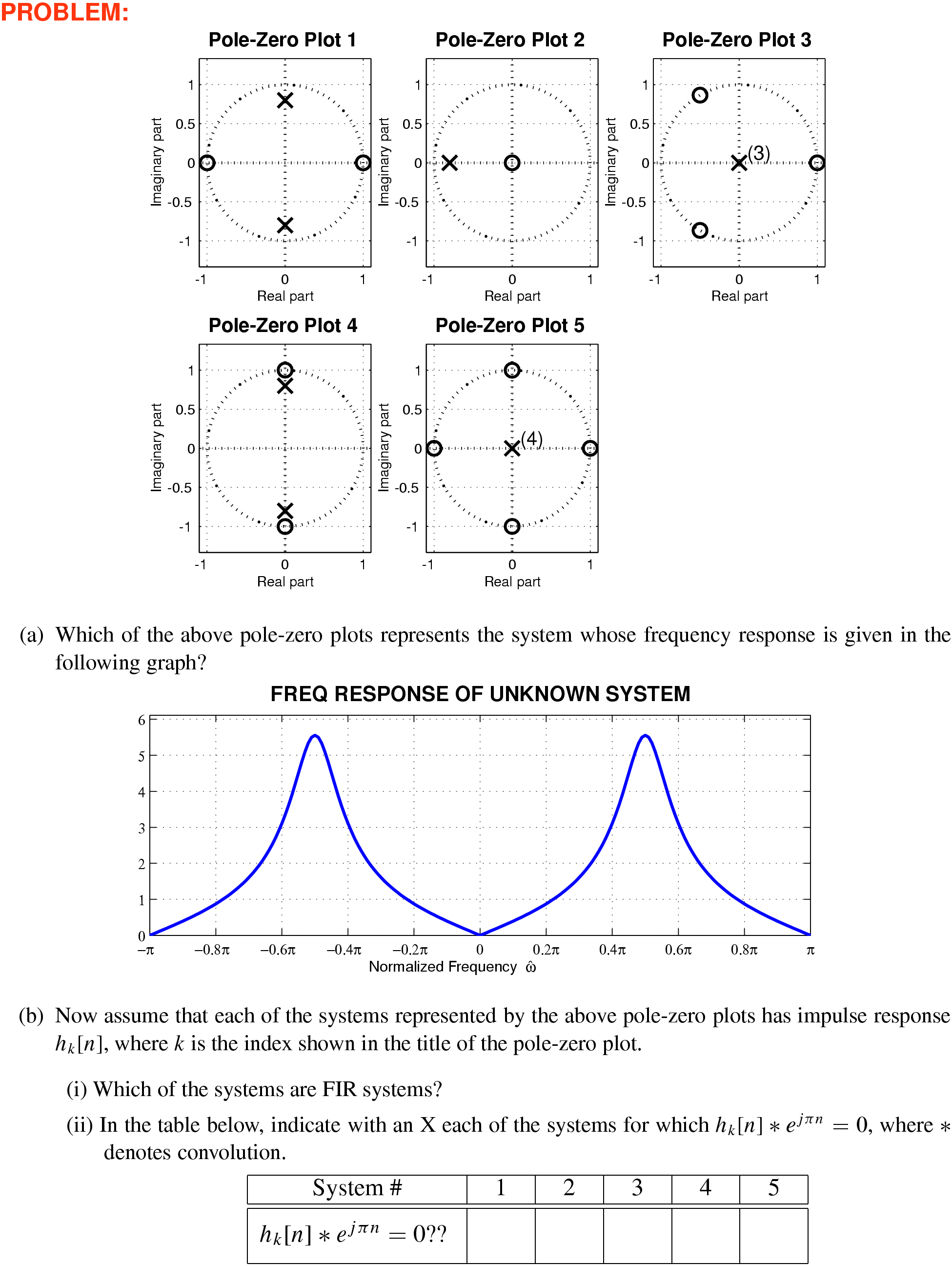
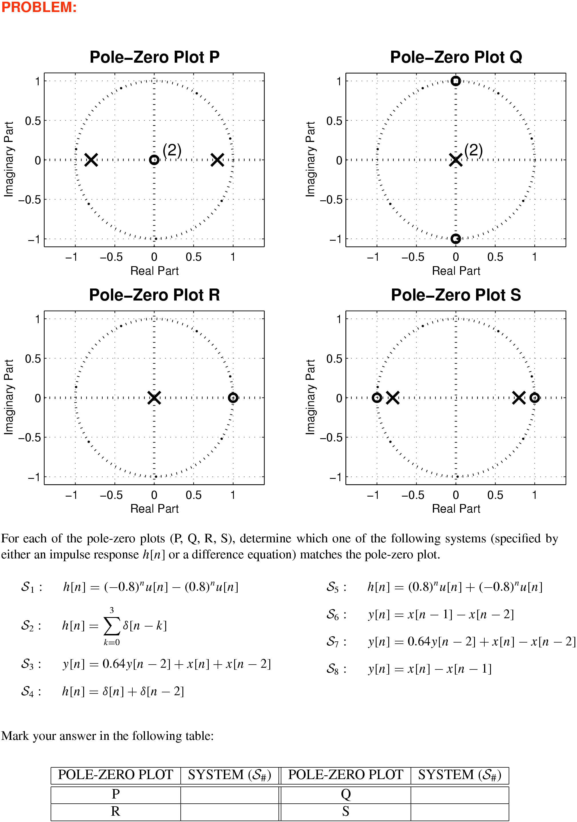
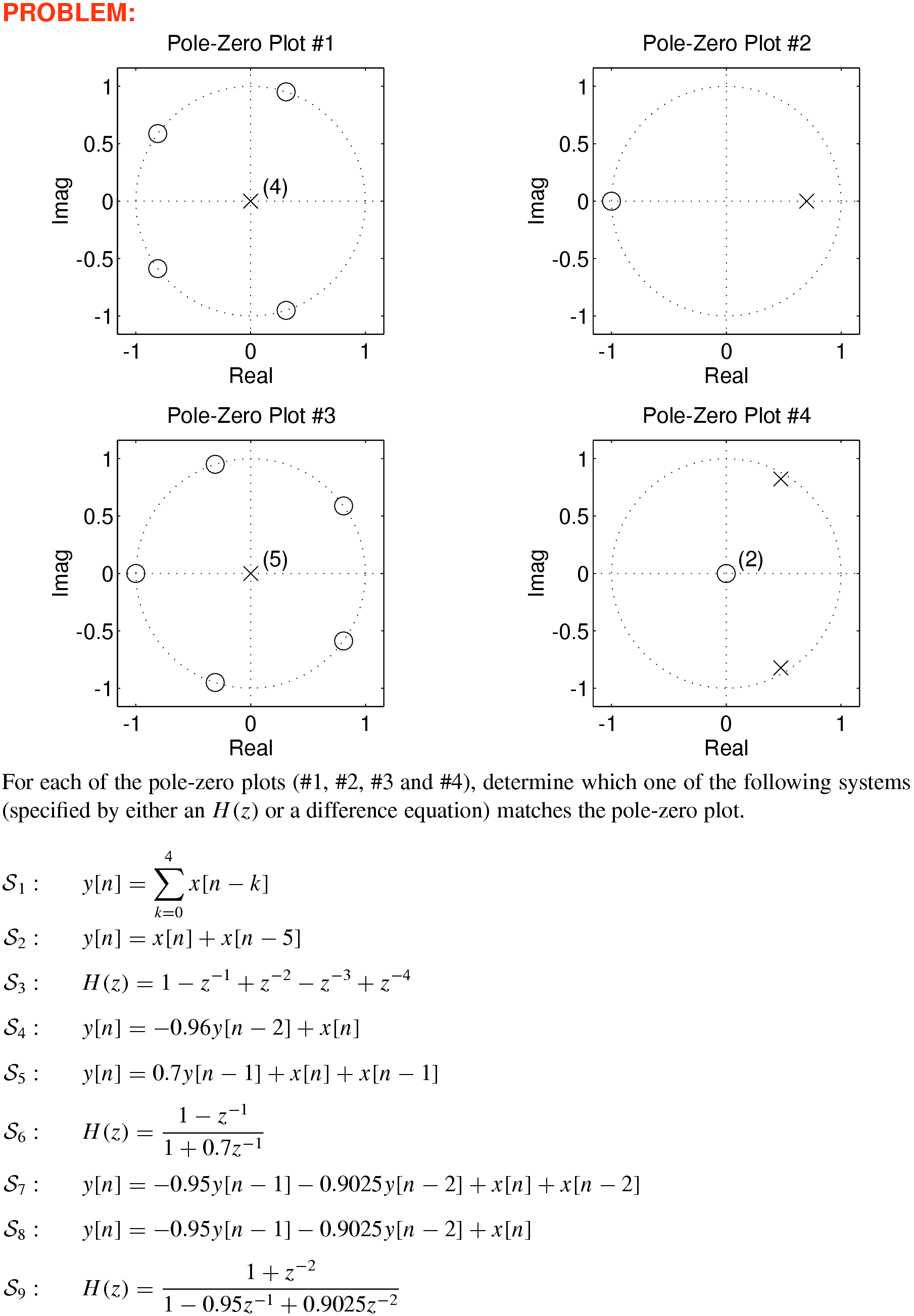
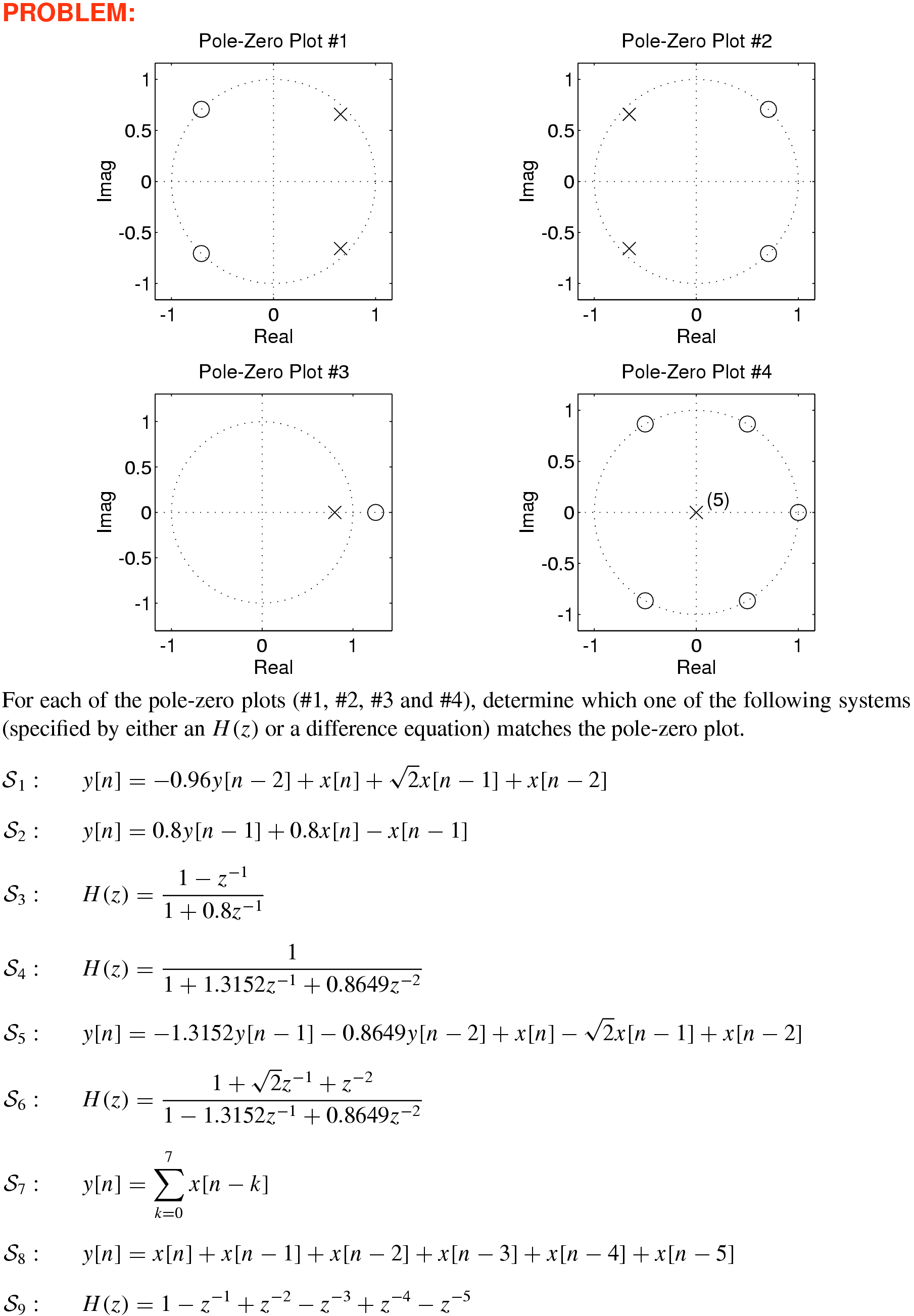
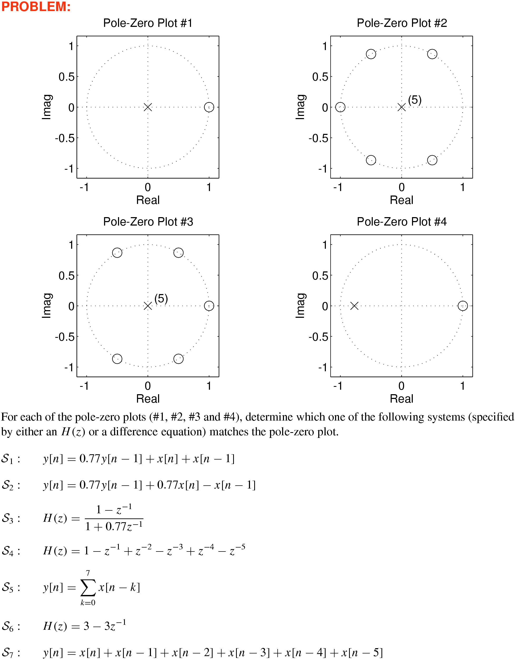
–24 Matching Pole-Zero Plots to Various \(H(z)\) and Difference Equations
Solution
10
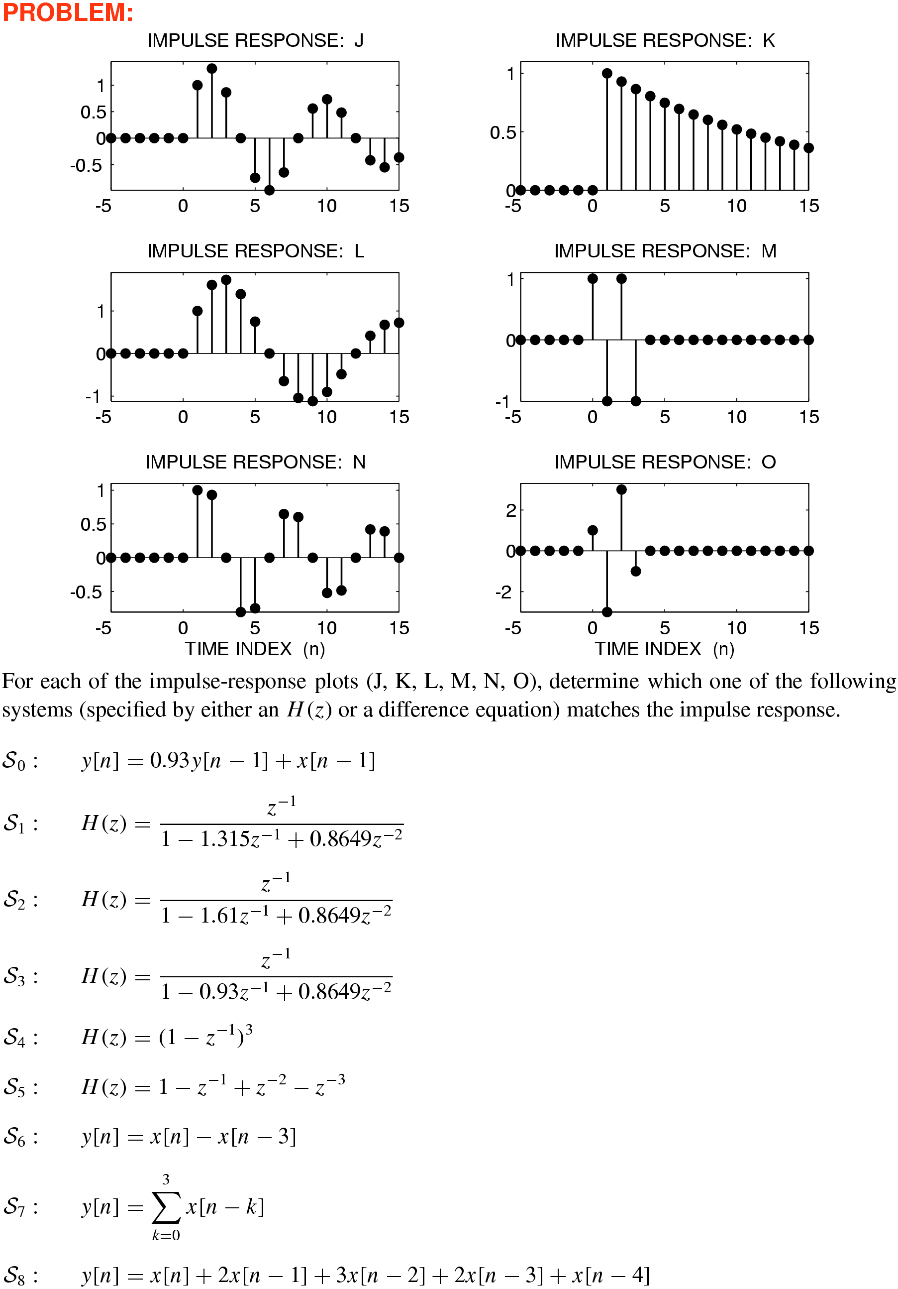
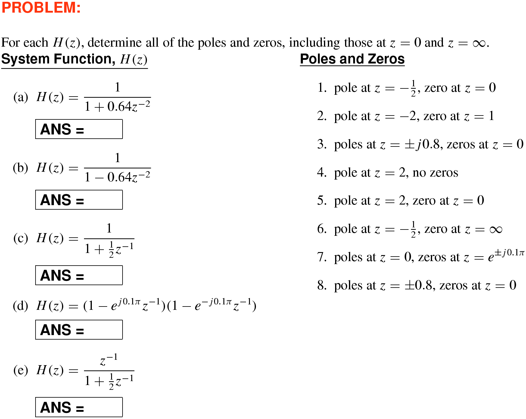
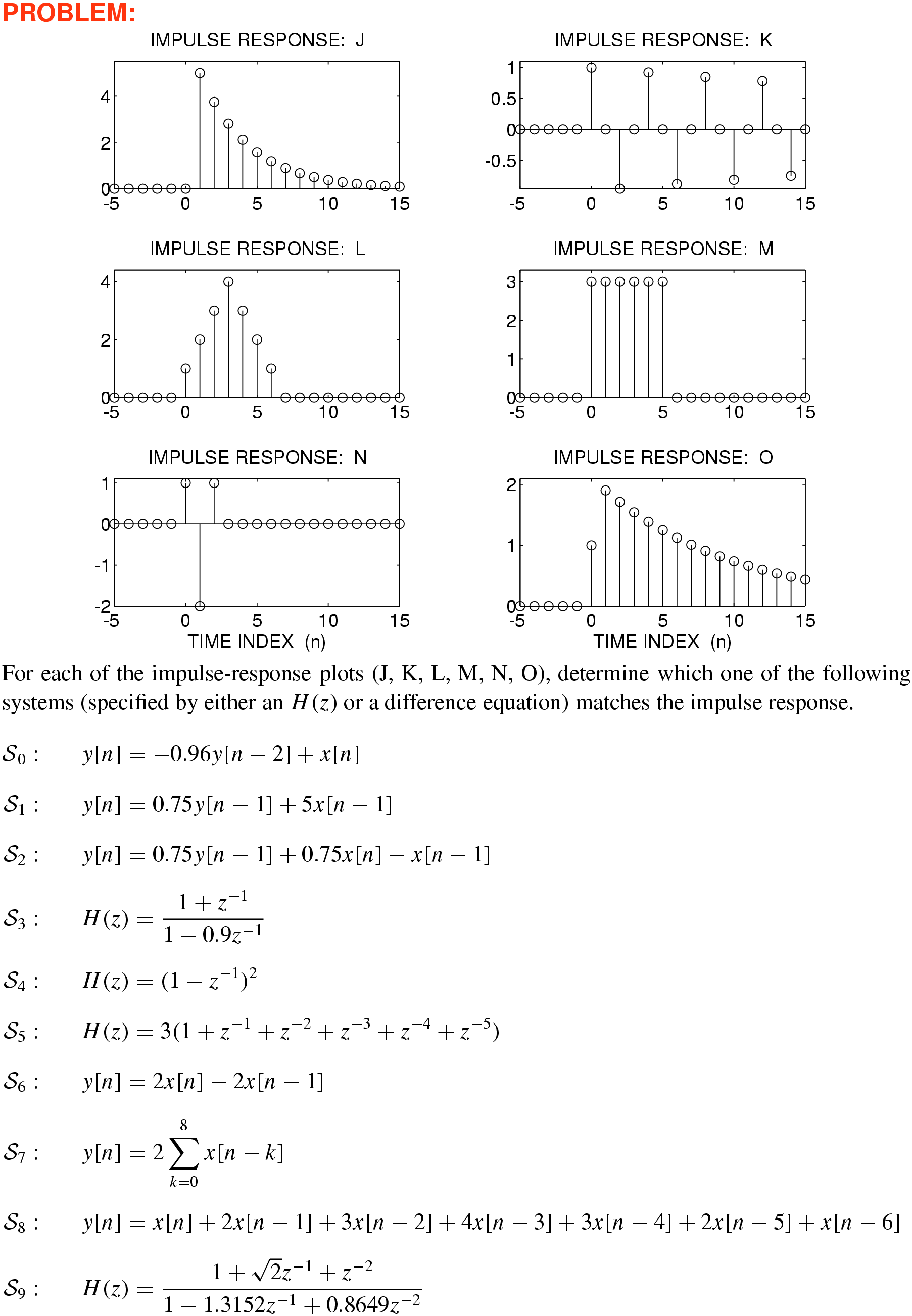
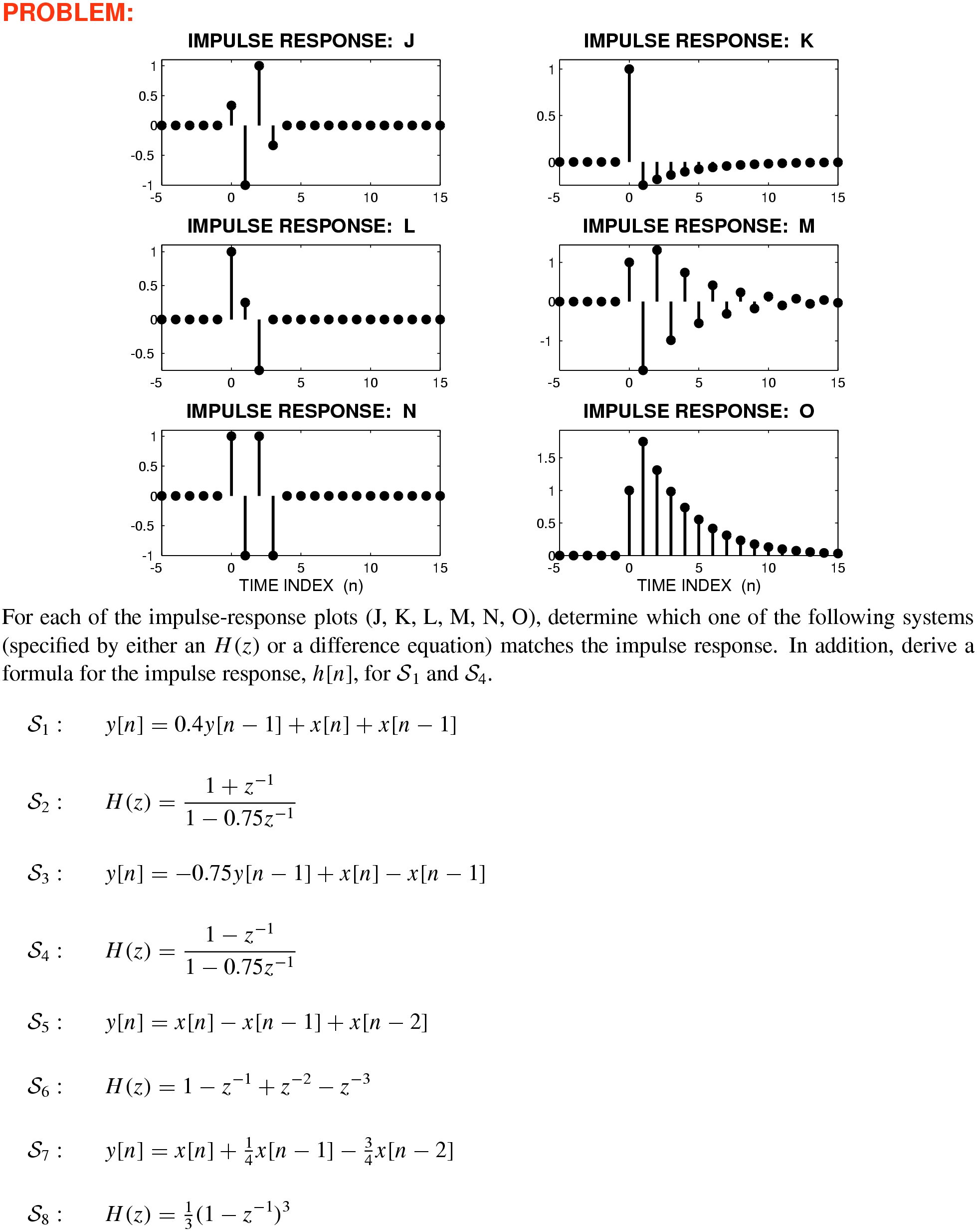
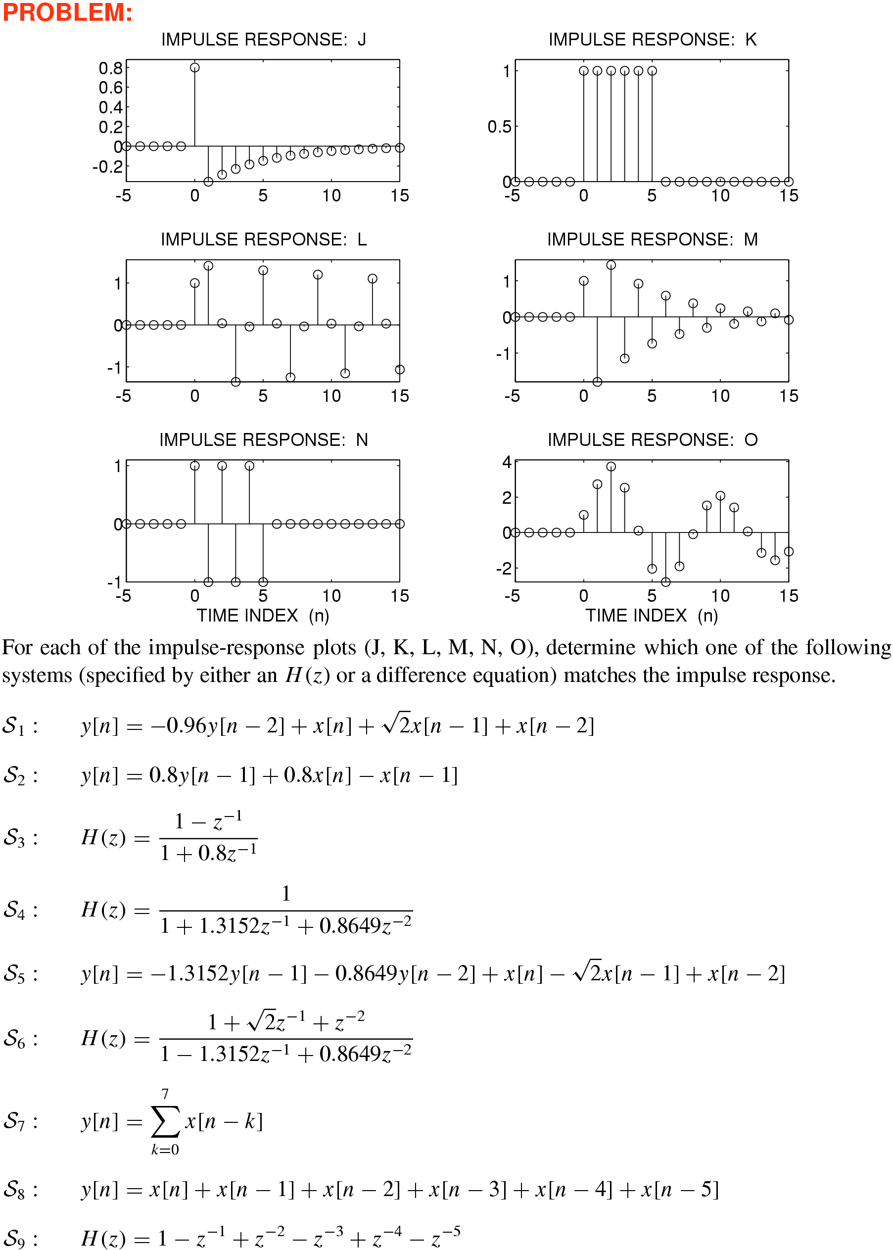
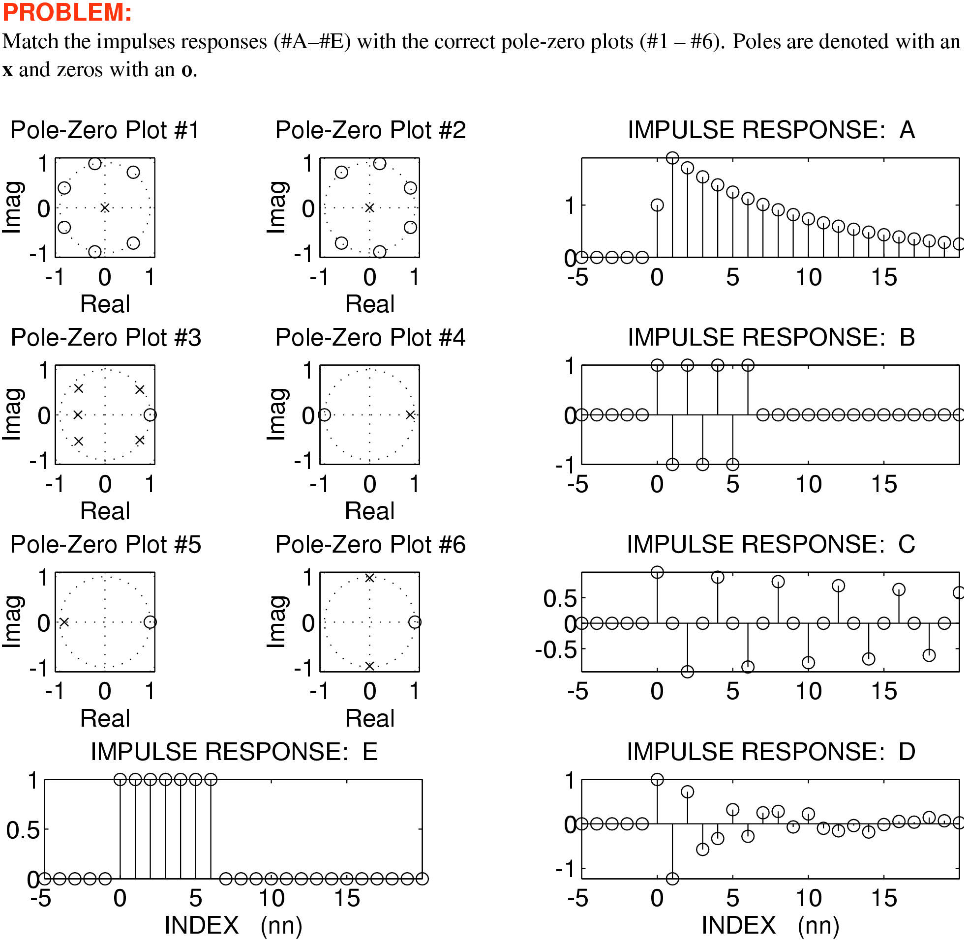
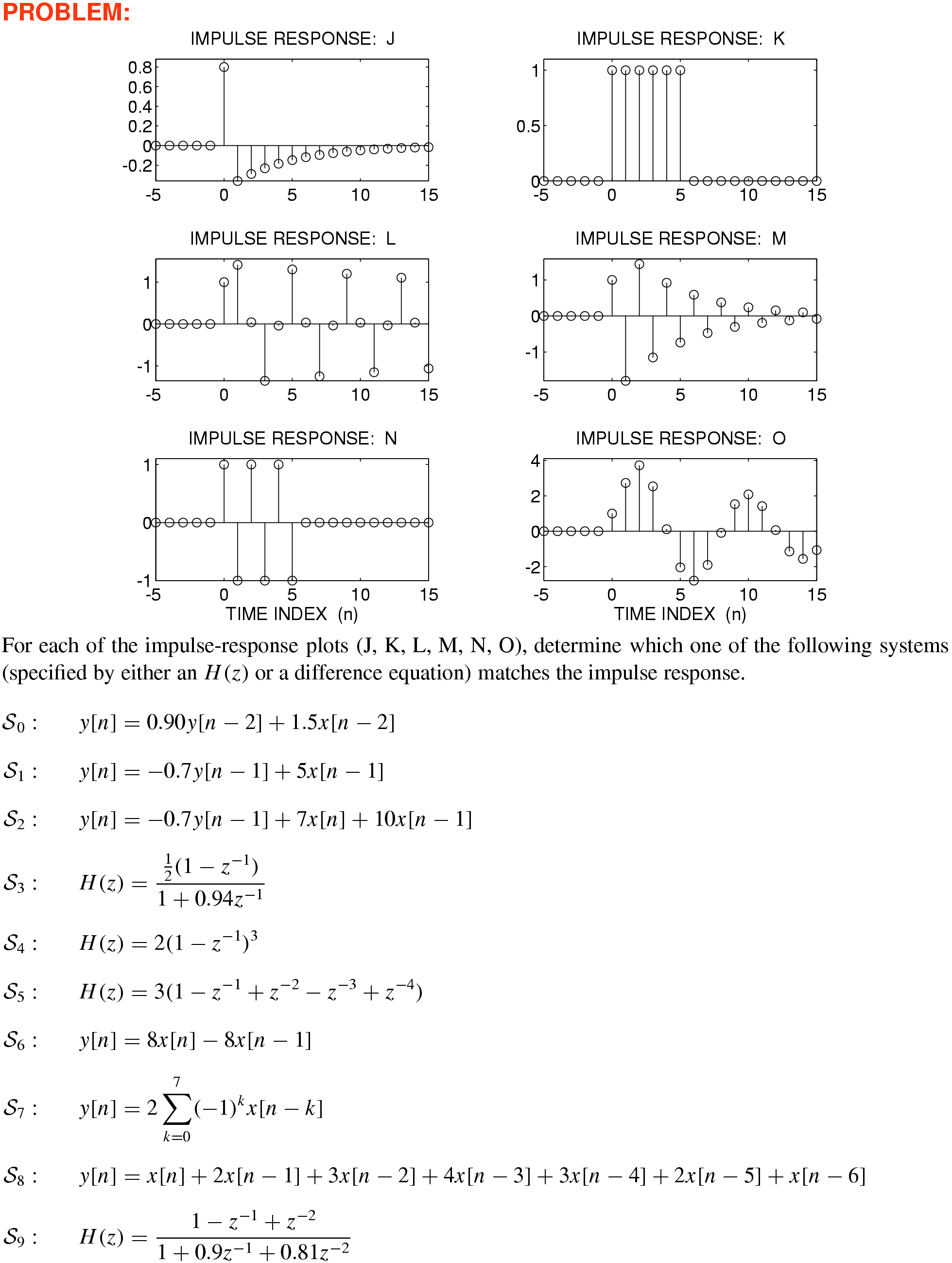
–25 Matching Impulse Responses \(h[n]\) to Various \(H(z)\) and Difference Equations
Solution
10
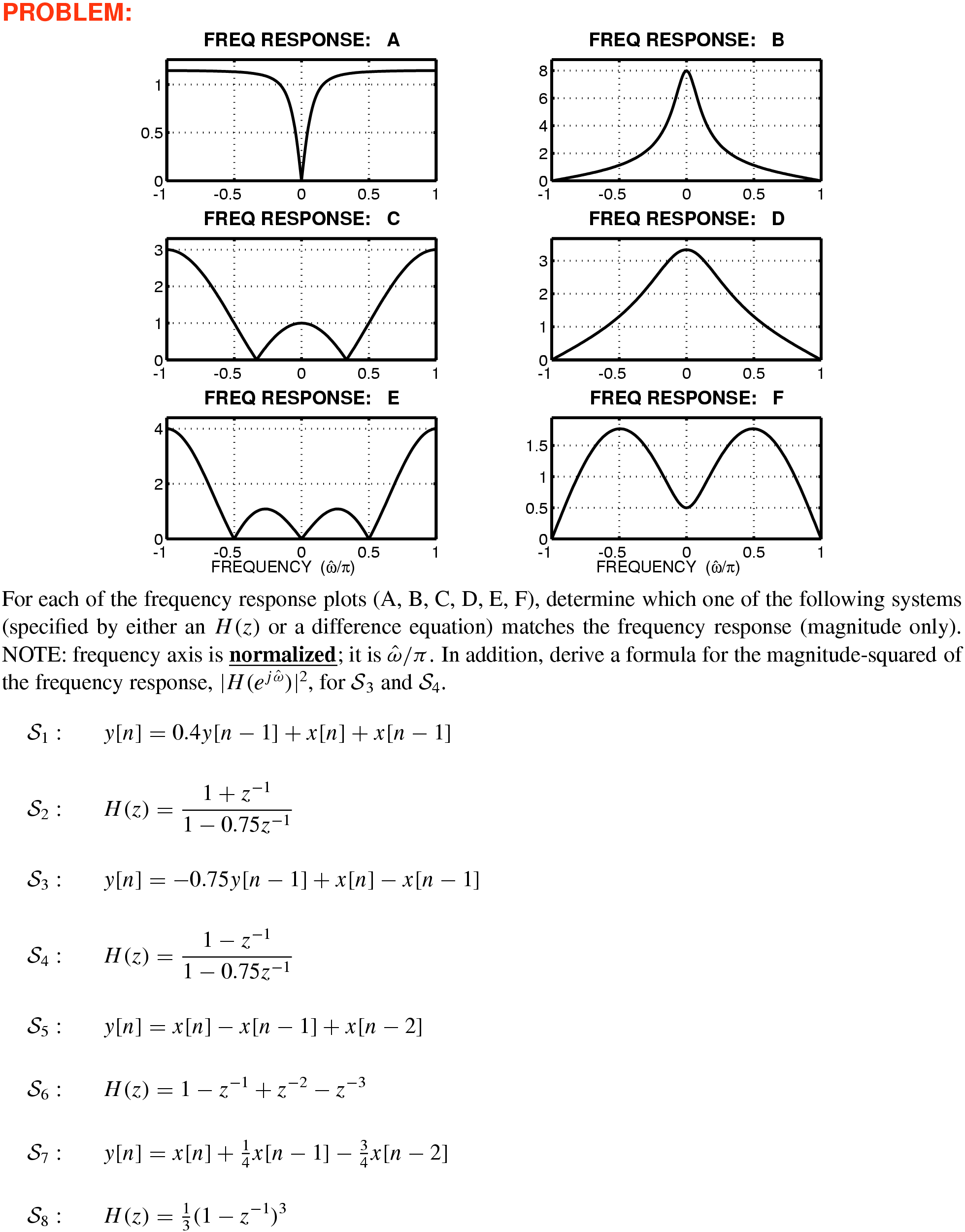
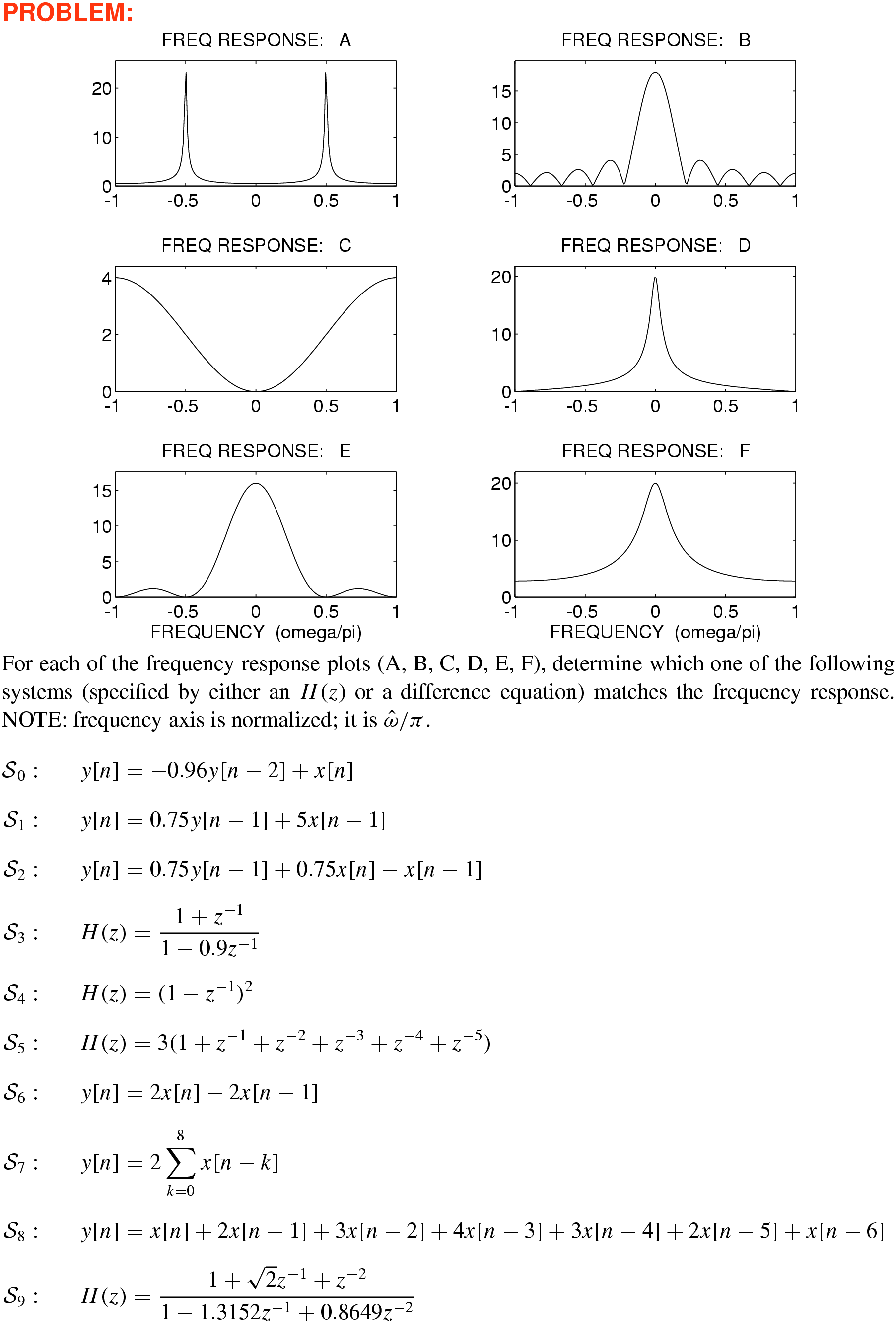
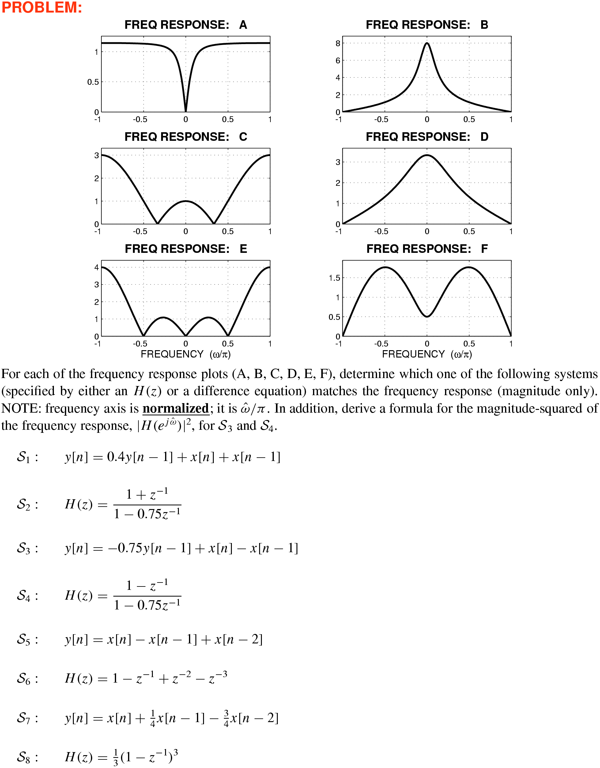
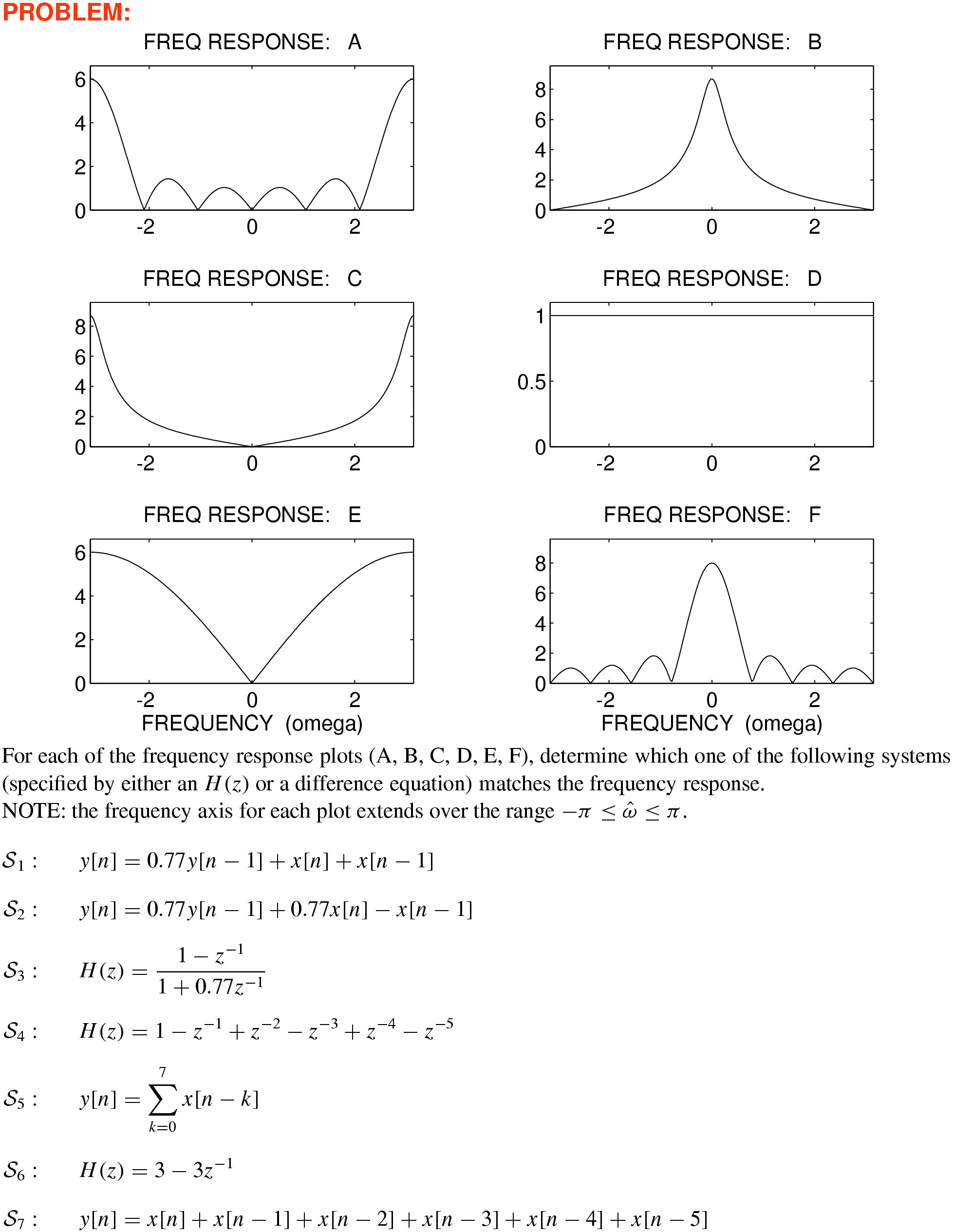
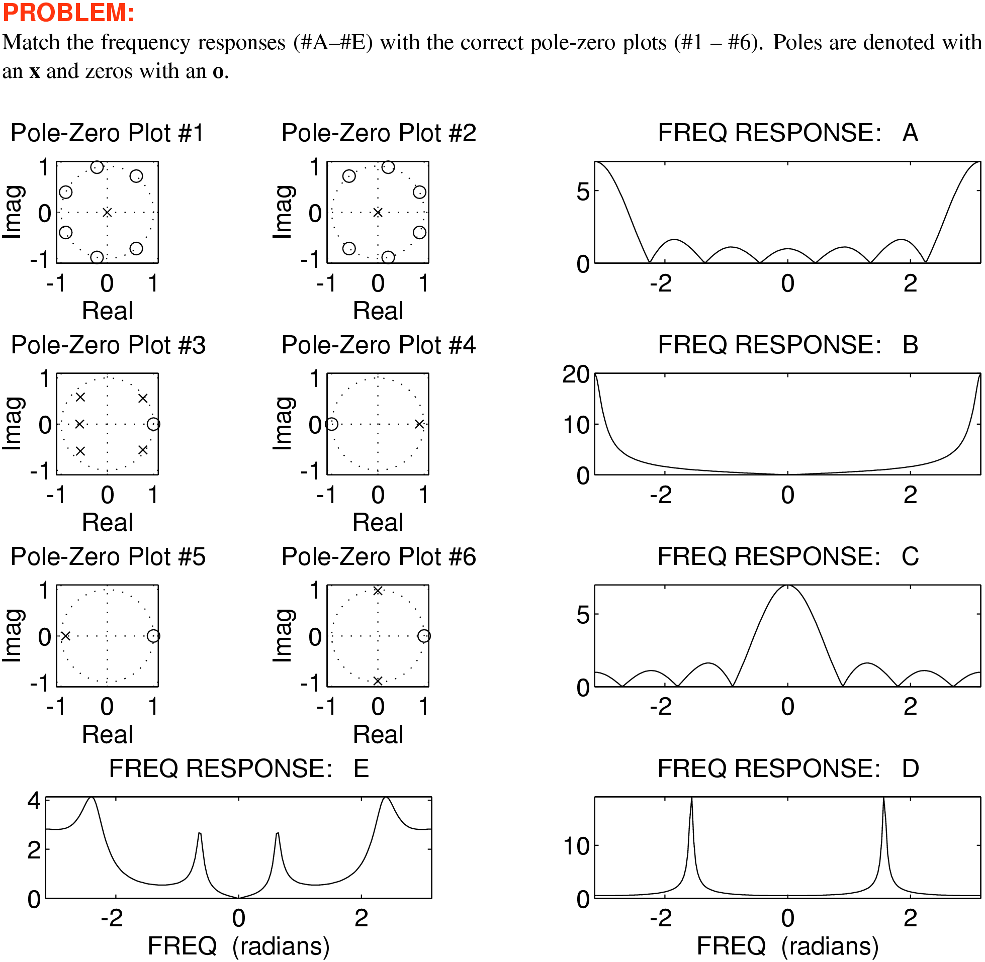
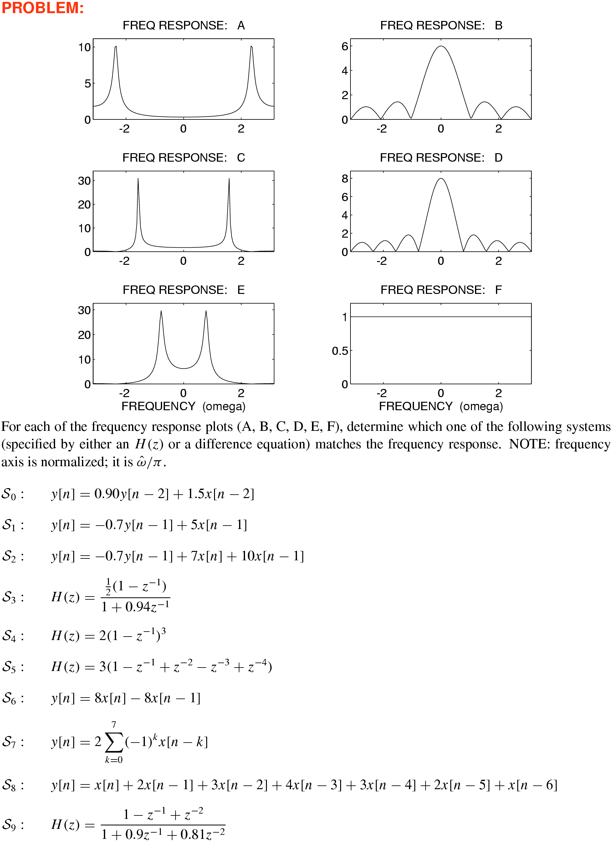
–26 Matching Frequency Responses to Various \(H(z)\) and Difference Equations
Solution
10
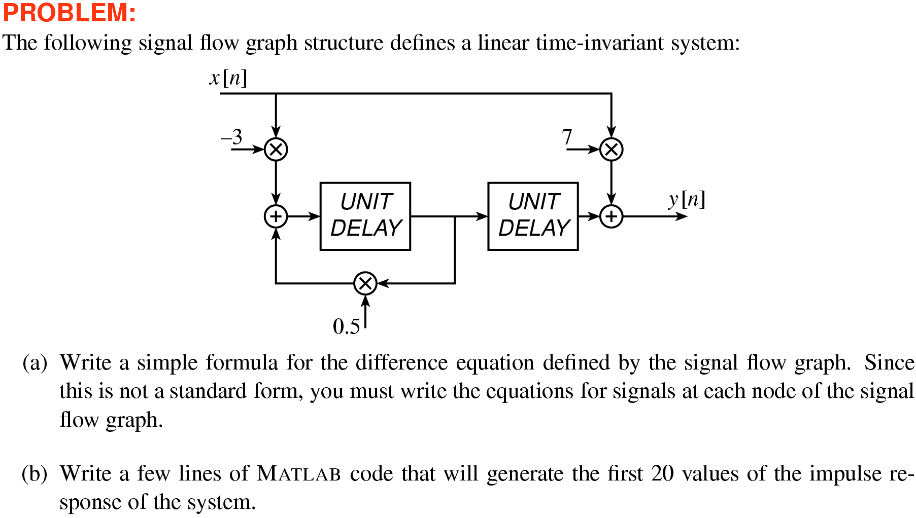
–27 Difference Equation Derived from Block Diagram of IIR Filter
Solution
10
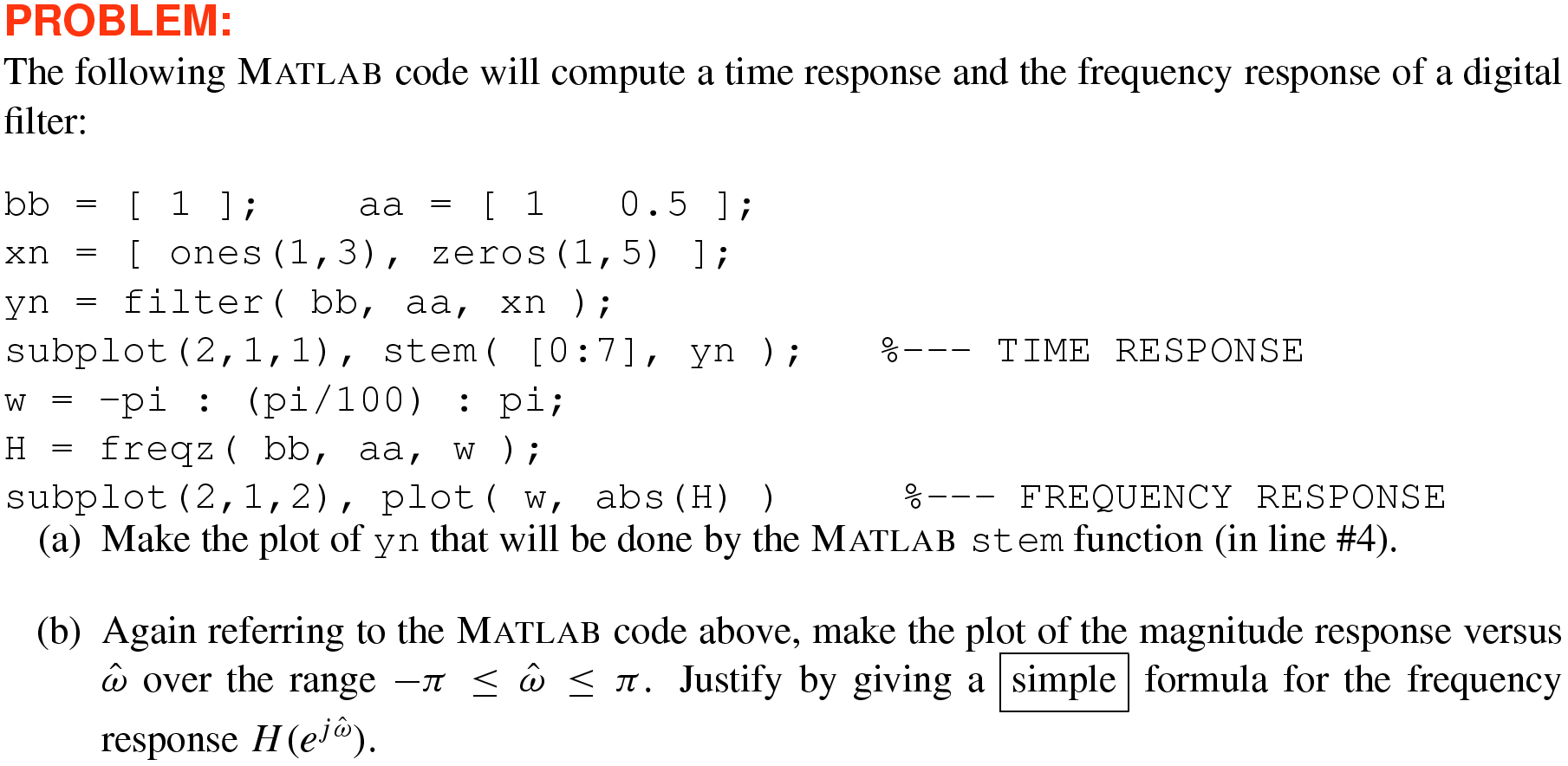
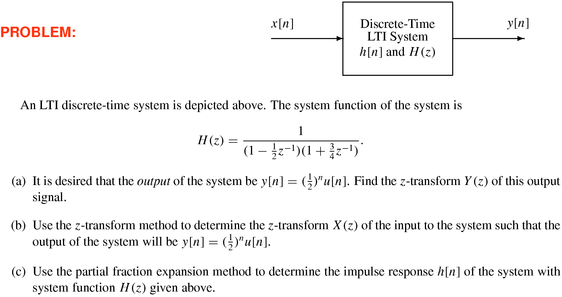
–28 Output Signal & Frequency Response for IIR Filter Defined by MATLAB Code
Solution
10
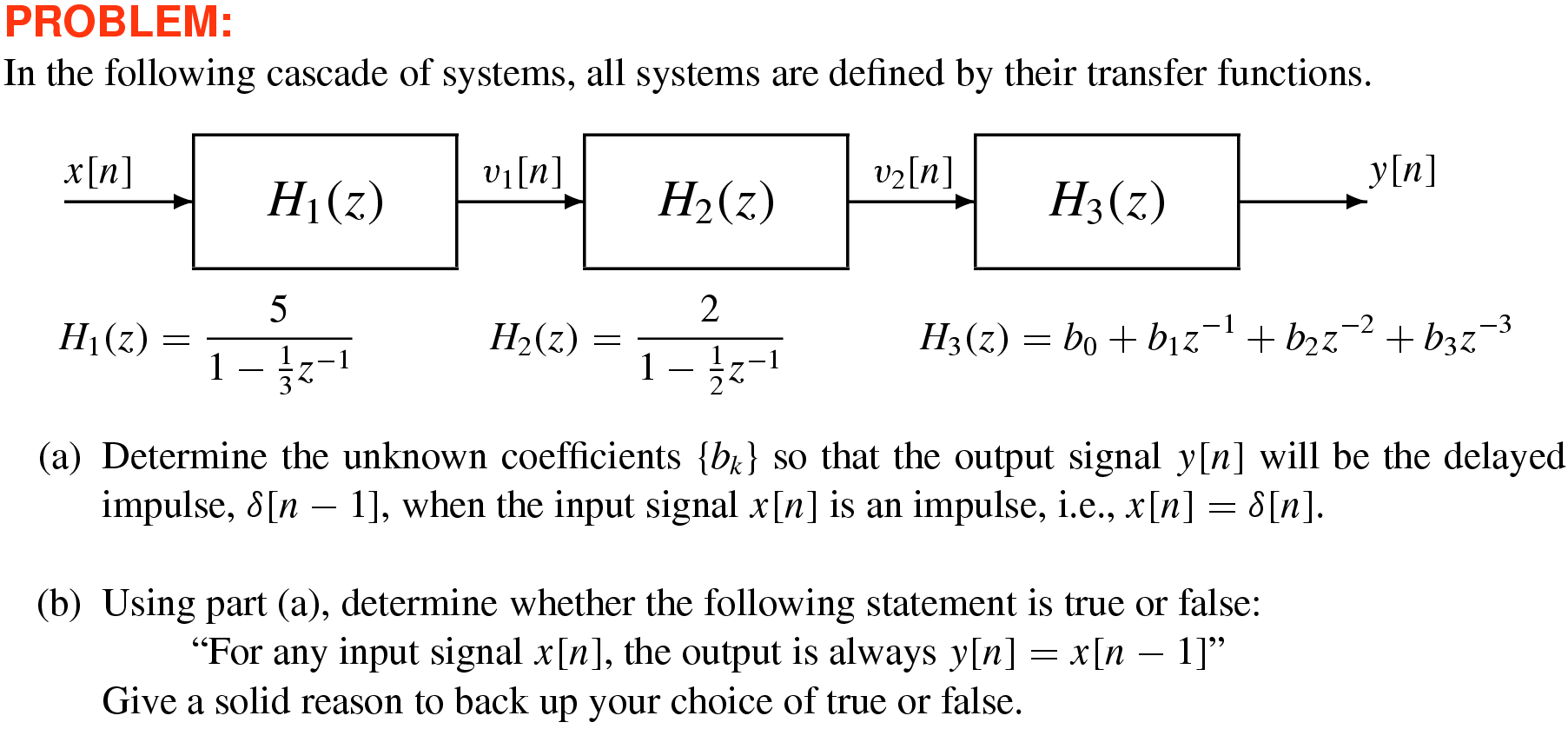
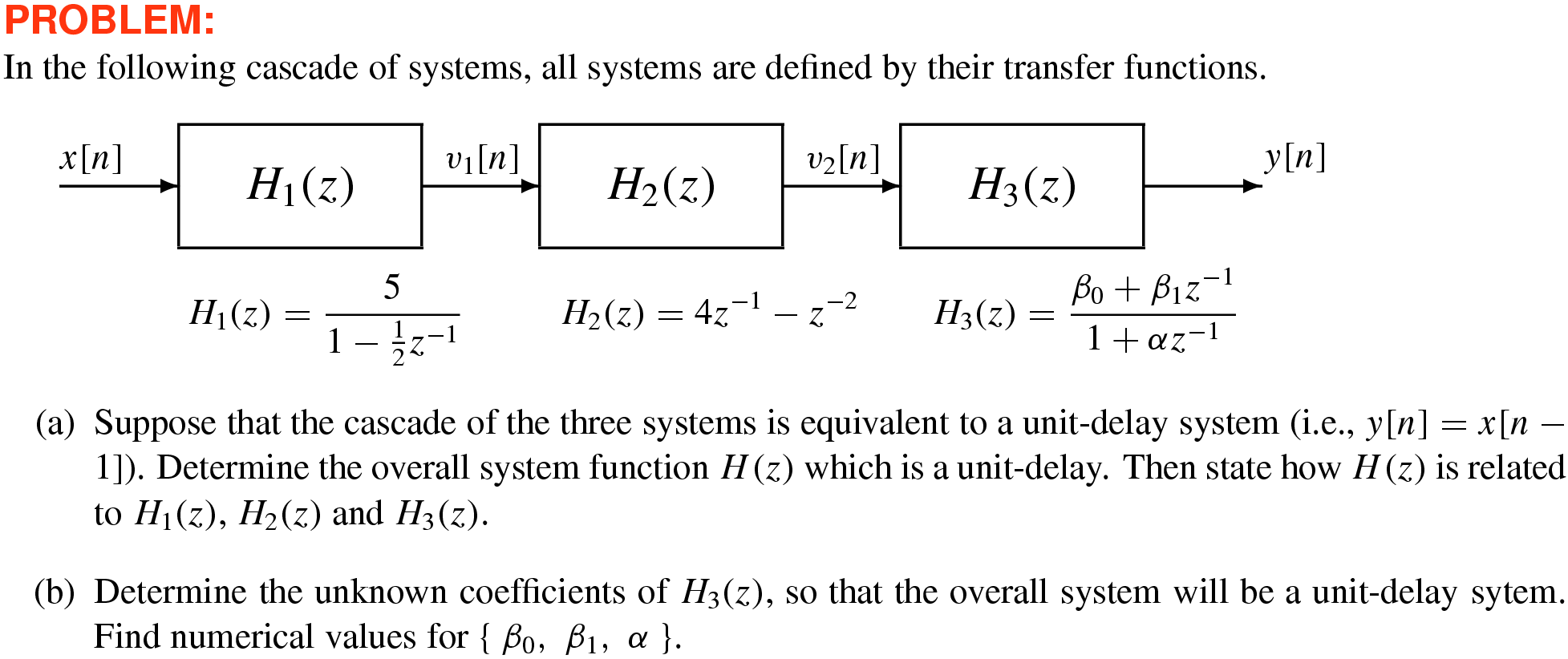
–29 Cascade of 3 LTI Systems ♦ \(H(z)\)
Solution
10
–30 \(H(z)\) for All-Pass IIR Filter ♦ Poles & Zeros ♦ Frequency Response
Solution
10
–31 Difference Equation from Rational \(H(z)\) ♦ Zeros & Poles
Solution
10
–32 \(H(z)\) from IIR Difference Equation ♦ Frequency Response ♦ Poles & Zeros
Solution
10
–33 Design IIR Filter \(H(z)\) to Synthesize \(y[n]\)
Solution
10
–34 \(H(z)\) from IIR Difference Equation ♦ Poles & Zeros ♦ Output Signal
Solution
10
–35 \(H(z)\) from IIR Difference Equation ♦ Poles & Zeros
Solution
10
–36 \(H(z)\) from IIR Difference Equation ♦ Frequency Response ♦ Nulling
Solution
10
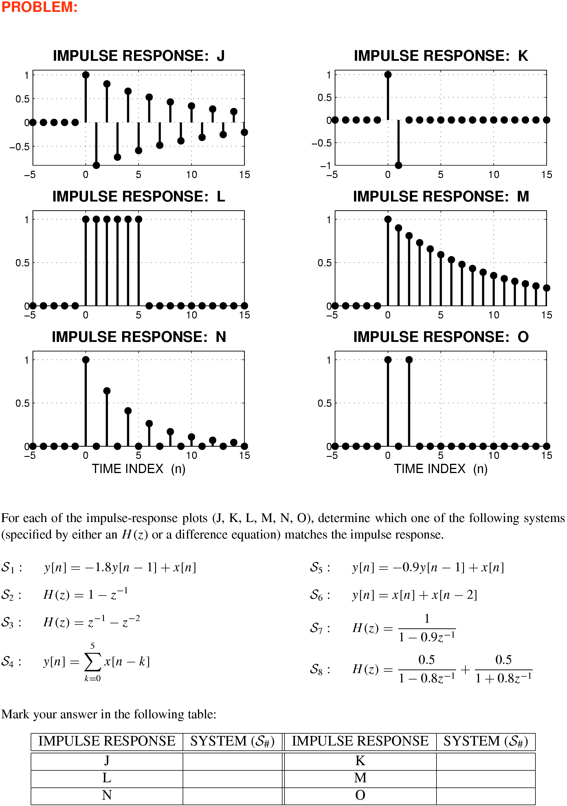
–37 Matching Impulse Responses \(h[n]\) to Various \(H(z)\) and Difference Equations
Solution
10
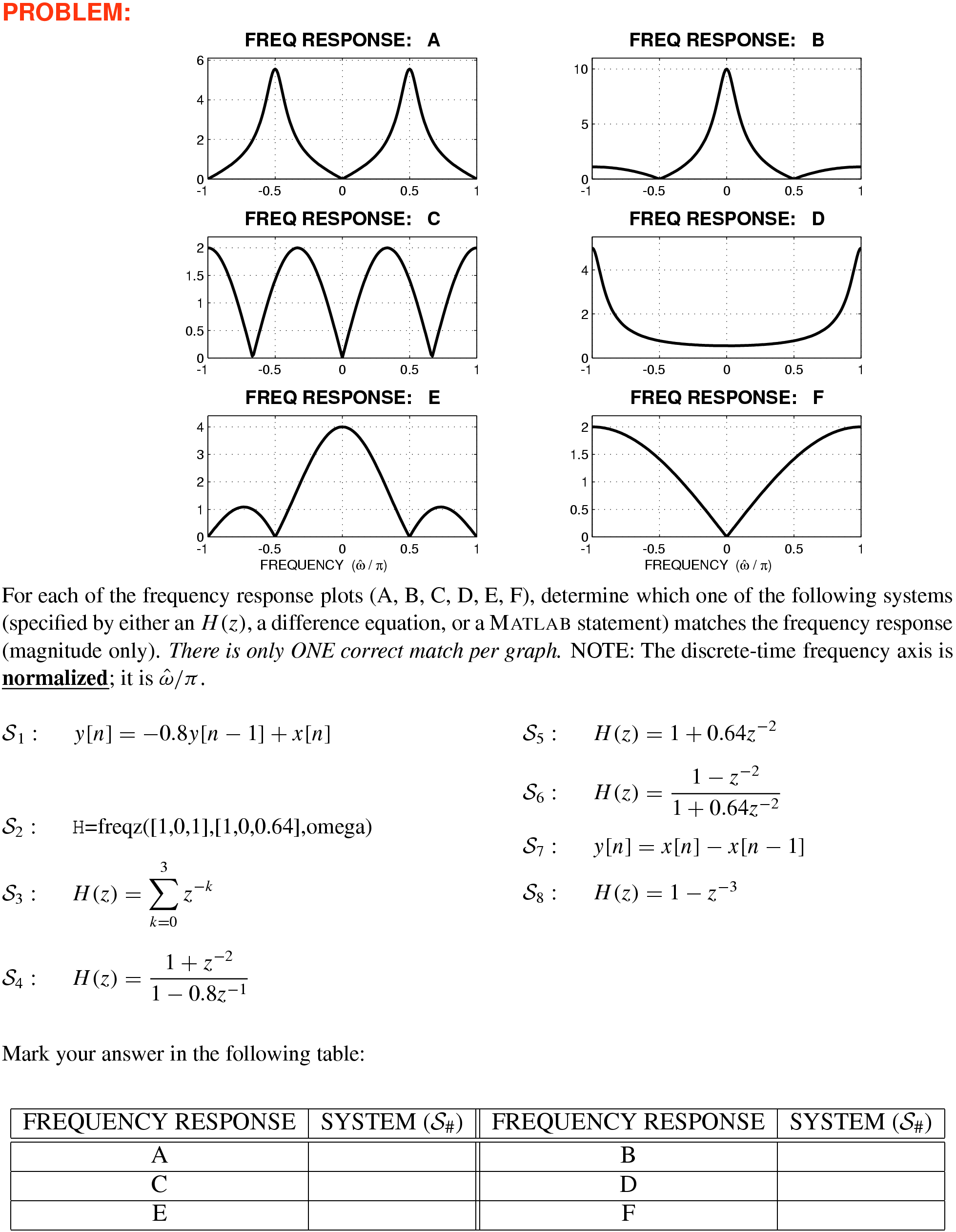
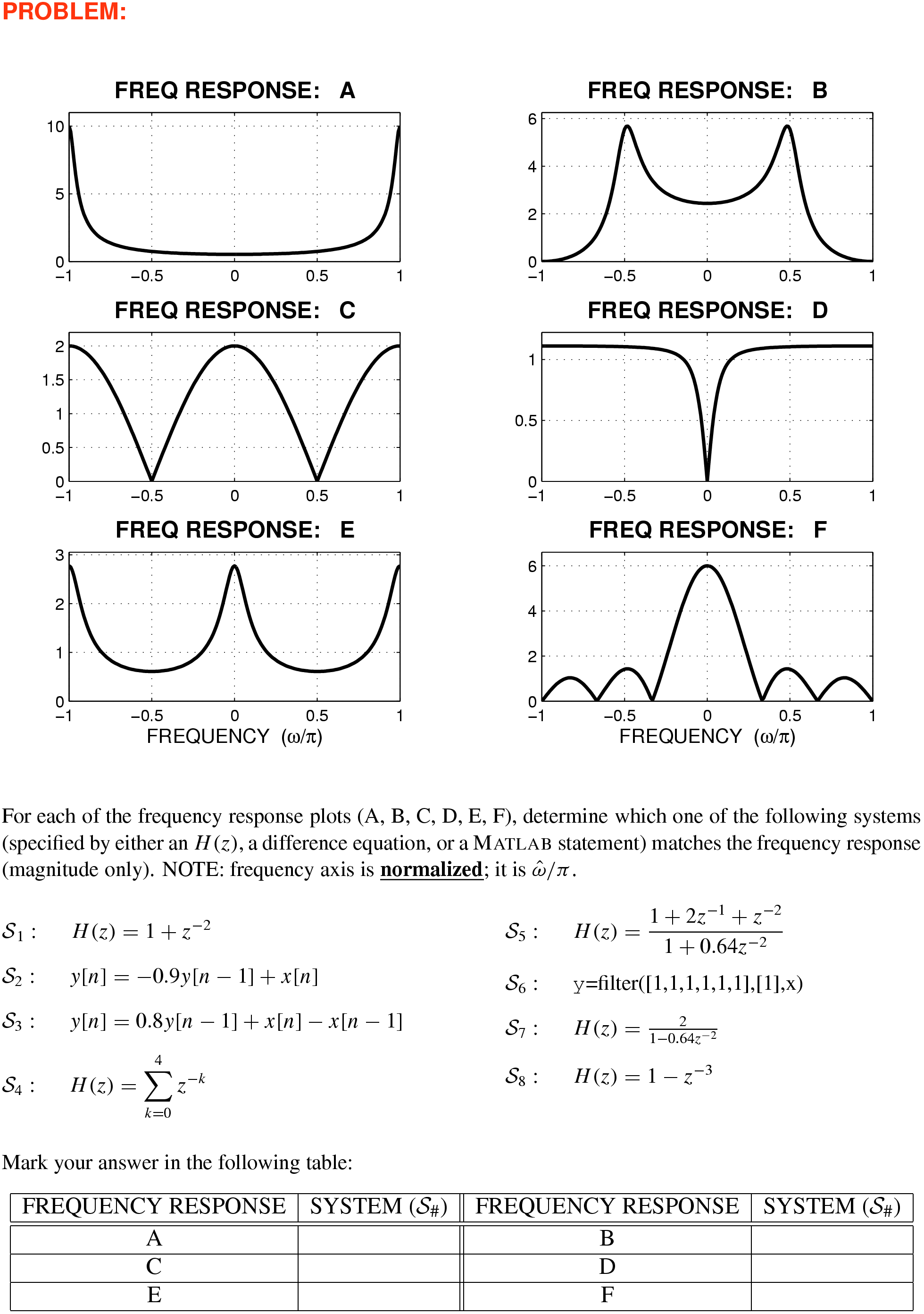
–38 Matching Frequency Responses to Various \(H(z)\) and Difference Equations
Solution
10
–39 Poles & Zeros from Difference Equation and \(H(z)\)
Solution
10
–40 Cascade of 3 LTI Systems ♦ \(H(z)\) ♦ Impulse Response
Solution
10
–41 Cascade of 2 Systems: FIR & IIR ♦ Impulse Response
Solution
10
–42 Cascade of 2 Systems: FIR & IIR ♦ Poles & Zeros ♦ Complex Exponential Input
Solution
10
–43 Cascade of 2 Systems: FIR & IIR ♦ \(H(z)\) ♦ Difference Equation
Solution
10
–44 Output Signal & Frequency Response for IIR Filter from \(h[n]\) and \(x[n]\)
Solution
10
–45 \(H(z)\) from MATLAB Code for IIR Filter ♦ Block Diagram ♦ Impulse Response
Solution
10
–46 Pole-Zero Plot Derived from Impulse Response and Frequency Response
Solution
10
–47 Matching Impulse Response \(h[n]\) to \(H(z)\) or Difference Equation
Solution
10
–48 Matching Frequency Response to \(H(z)\) or Difference Equation
Solution
10
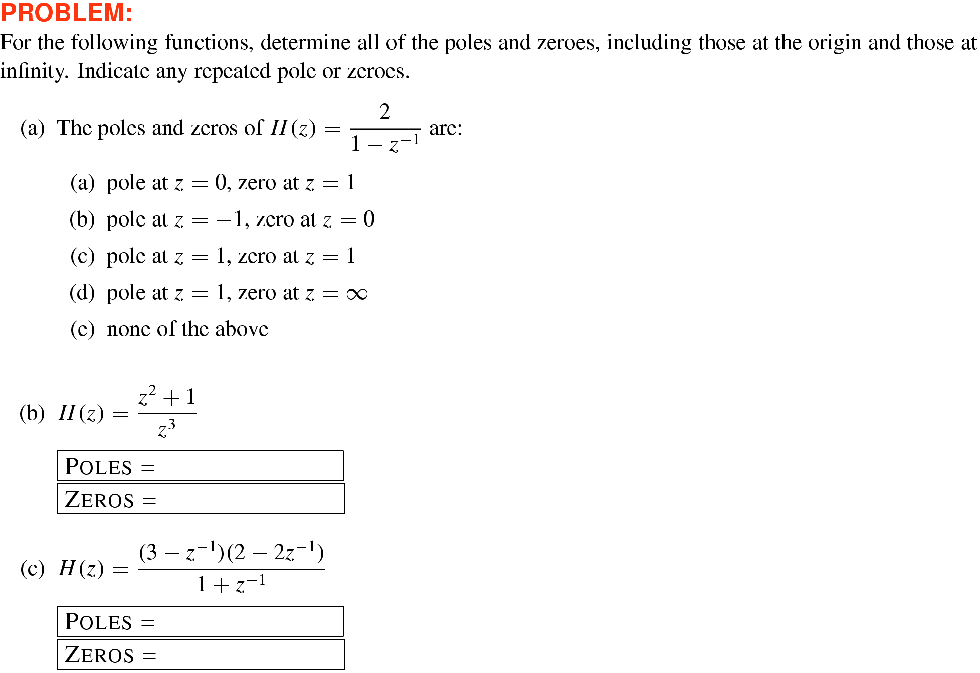
–49 Poles and Zeros of \(H(z)\)
Solution
10
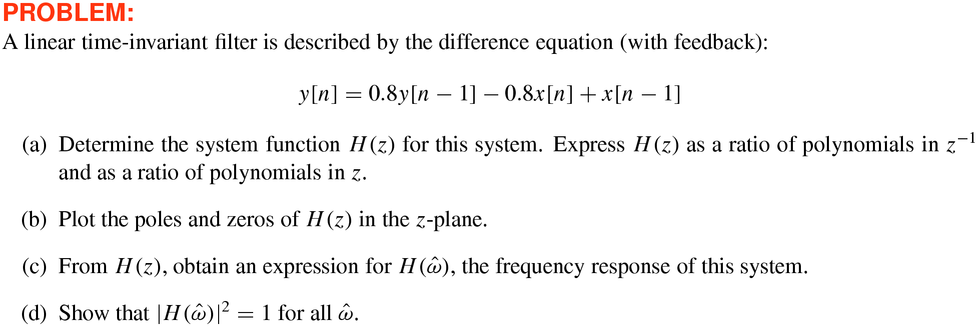
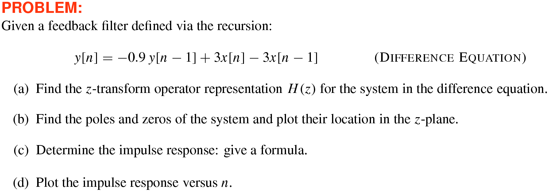
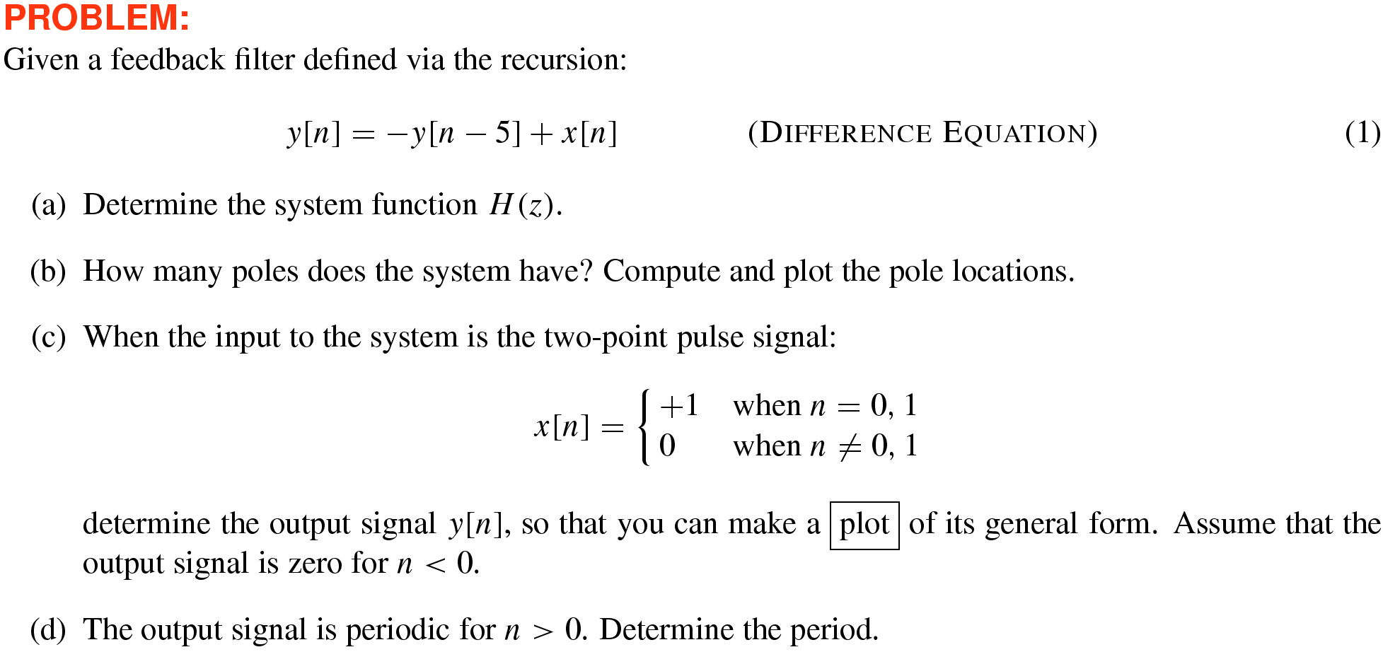
–50 Output and Impulse Response for Feedback Filter
10
–51 Inverse \(z\mbox{-}\)Transform & Frequency Response from \(H(z)\)
10
–52 \(H(z)\) & Frequency Response from IIR Difference Equation
10
–53 Find Output via Inverse \(z\mbox{-}\)Transform of System Function
10
–54 Cascade of 3 LTI Systems ♦ \(H(z)\) ♦ Impulse Response
10
–55 Match the Impulse Response with \(H(z)\) or the Difference Equation
10
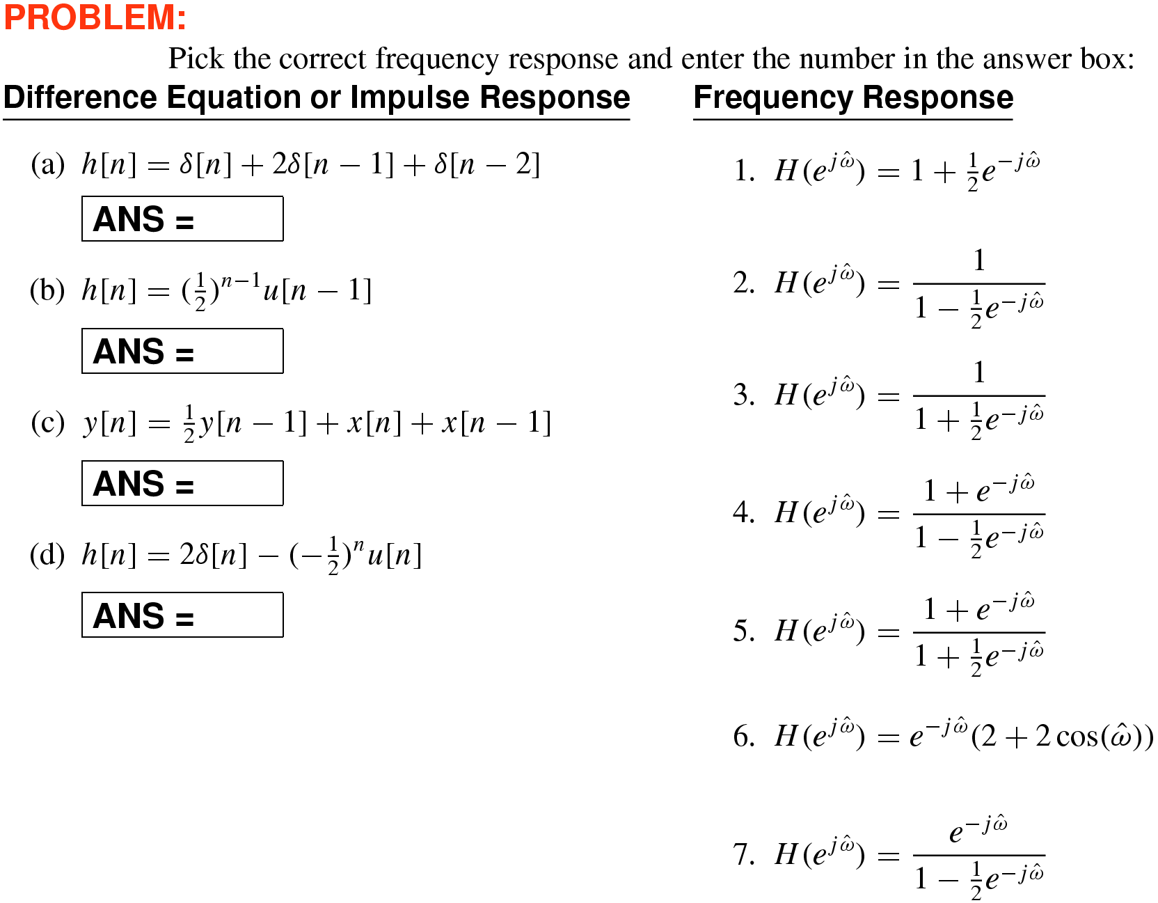
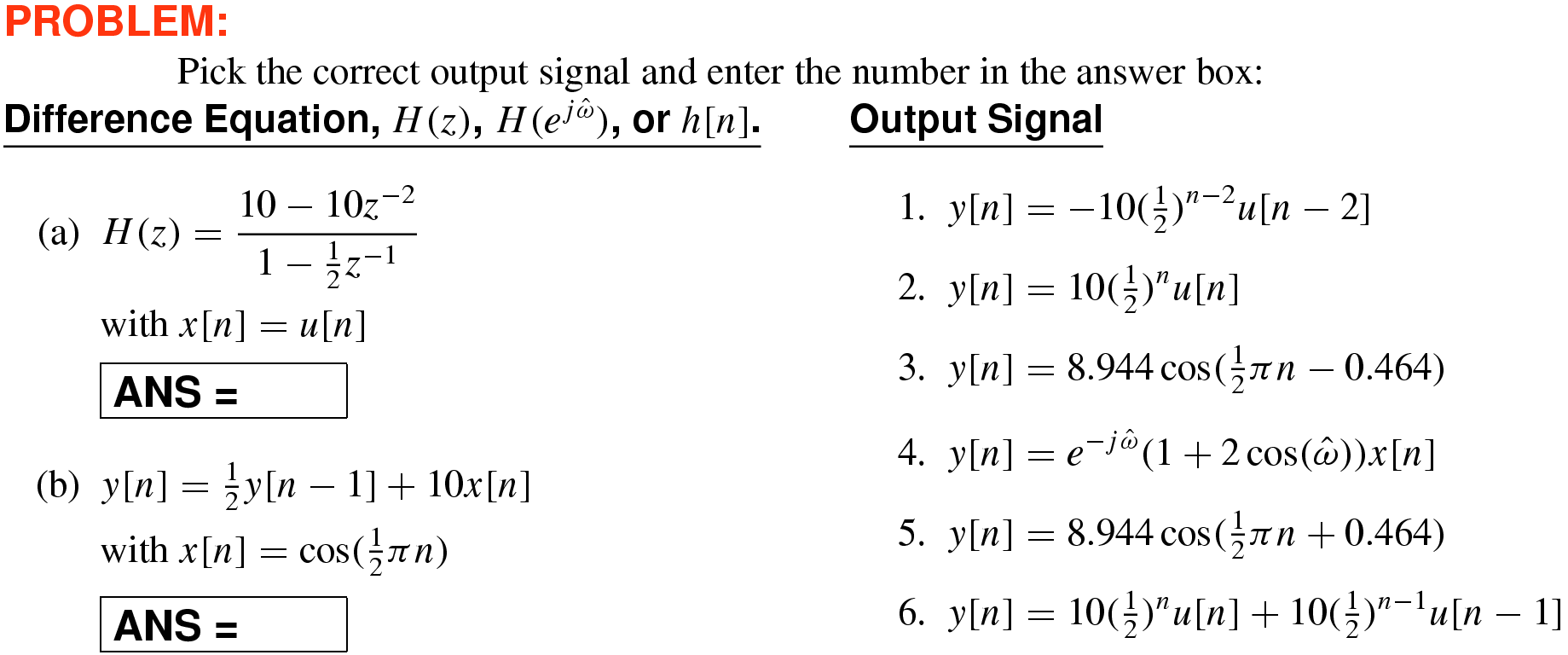
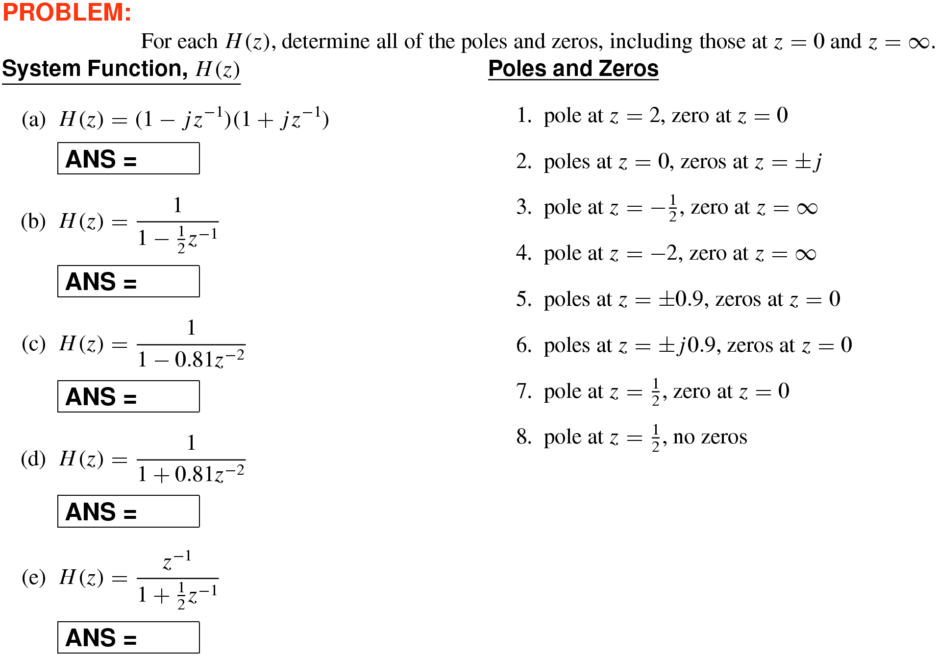
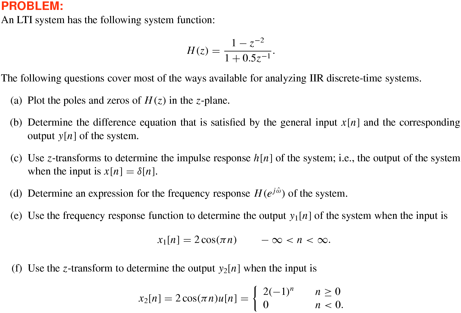
–56 Match the Frequency Response with \(H(z)\) or the Difference Equation
10
–57 Pole-zero plot of system function
Solution
10
–58 Output signal via \(z\mbox{-}\)transform method
Solution
10
–59 Pole-zero plot of system function
10
–60 Output signal via \(z\mbox{-}\)transform method
10
–61 Pole-zero plot of system function
10
–62 Output signal via \(z\mbox{-}\)transform method
10
–63 Matching impulse responses
Solution
10
–64 Matching frequency responses
Solution
10
–65 3 Domains for IIR filter
Solution
10
–66 Matching impulse responses
10
–67 Matching frequency responses
10
–68 3 Domains for IIR filter
10
–69 Matching impulse responses
10
–70 Matching frequency responses
10
–71 3 Domains for IIR filter
10
–72 Matching poles and zeros from difference equation
10
–73 Matching impulse responses
10
–74 Matching frequency responses
10
–75 Difference equation and poles and zeros from \(H(z)\)
Solution
10
–76 Impulse and Frequency response from \(H(z)\)
Solution
10
–77 Difference equation and poles and zeros from \(H(z)\)
Solution
10
–78 Impulse and Frequency response from \(H(z)\)
Solution
10
–79 Difference equation and poles and zeros from \(H(z)\)
Solution
10
–80 Impulse and Frequency response from \(H(z)\)
Solution
10
–81 Frequency Response from FIR Difference Equation or Impulse Response
Solution
10
–82 Output From System Function or Difference Equation
Solution
10
–83 Poles and Zeros of \(H(z)\)
Solution
10
–84 Frequency Response from FIR Difference Equation or Impulse Response
Solution
10
–85 Output From System Function or Difference Equation
Solution
10
–86 Poles and Zeros of \(H(z)\)
Solution
10
–87 Frequency Response from FIR Difference Equation or Impulse Response
Solution
10
–88 Output From System Function or Difference Equation
Solution
10
–89 Poles and Zeros of \(H(z)\)
Solution
10
–90 Compute the Output of an IIR System
Solution
10
–91 Match the Impulse Response with \(H(z)\) or the Difference Equation
Solution
10
–92 Match the Frequency Response with \(H(z)\) or the Difference Equation
Solution
10
–93 Cascade of Two Discrete-Time Systems ♦ Find \(H(z)\)
Solution
10
–94 Matching Frequency Responses of a Discrete-Time System to Other Descriptions
Solution
10
–95 Matching Pole-Zero Plots to Other Descriptions of a System
Solution
10
–96 Cascade of Two Discrete-Time Systems ♦ Find \(H(z)\)
Solution
10
–97 Matching Frequency Responses of a Discrete-Time System to Other Descriptions
Solution
10
–98 Matching Pole-Zero Plots to Other Descriptions of a System
Solution
10
–99 Cascade of Two Discrete-Time Systems ♦ Find \(H(z)\)
Solution
10
–100 Matching Frequency Responses of a Discrete-Time System to Other Descriptions
Solution
10
–101 Matching Pole-Zero Plots to Other Descriptions of a System
Solution
10
–102 \(z\mbox{-}\)Transform of IIR
Solution
10
–103 Which Domain Should You Use to Solve a Given Problem?
Solution
10
–104 Match the Impulse Response with \(H(z)\) or the Difference Equation
10
–105 Match the Frequency Response with \(H(z)\) or the Difference Equation
10
–106 Matching pole-zero plots to systems
Solution
10
–107 Matching pole-zero plots to systems
Solution
10
–108 Matching pole-zero plots to systems
Solution
10
–109 \(z\mbox{-}\)Transforms in rational form
Solution
10
–110 Poles & Zeros from Difference Equation and \(H(z)\)
Solution
10
–111 Matching Impulse Responses \(h[n]\) to Various \(H(z)\) and Difference Equations
Solution
10
–112 Matching Frequency Responses to Various \(H(z)\) and Difference Equations
Solution
10
–113 Sinusoidal Equations for IIR Filter Solved via Phasors
Solution
10
–114 Cascade of 3 LTI Systems ♦ \(H(z)\) ♦ Impulse Response
Solution
10
–115 Poles & Zeros from Difference Equation and \(H(z)\)
Solution
10
–116 Matching Impulse Responses \(h[n]\) to Various \(H(z)\) and Difference Equations
Solution
10
–117 Matching Frequency Responses to Various \(H(z)\) and Difference Equations
Solution
10
–118 Cascade of 3 LTI Systems ♦ \(H(z)\) ♦ Impulse Response
Solution
10
–119 \(H(z)\) from IIR Difference Equation ♦ Frequency Response ♦ Poles & Zeros
Solution
10
–120 Difference Equation from \(H(z)\) ♦ Frequency Response ♦ Poles & Zeros
Solution
10
–121 \(H(z)\) for All-Pass IIR Filter ♦ Poles & Zeros ♦ Frequency Response
Solution
10
–122 \(H(z)\) from IIR Difference Equation ♦ Impulse Response \(h[n]\) ♦ Poles & Zeros
Solution
10
–123 Frequency Response for FIR and IIR Filters
Solution
10
–124 Cascade of 3 LTI Systems ♦ \(H(z)\) ♦ Impulse Response
Solution
10
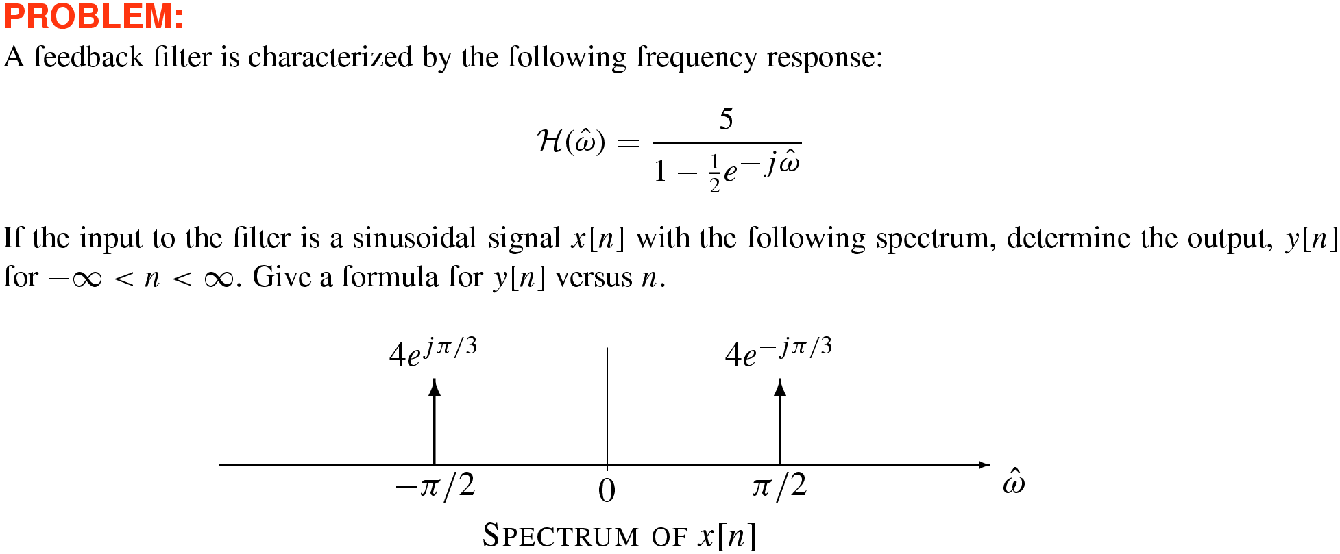
–125 Output Signal given Frequency Response of IIR Filter and Input Spectrum
Solution
10
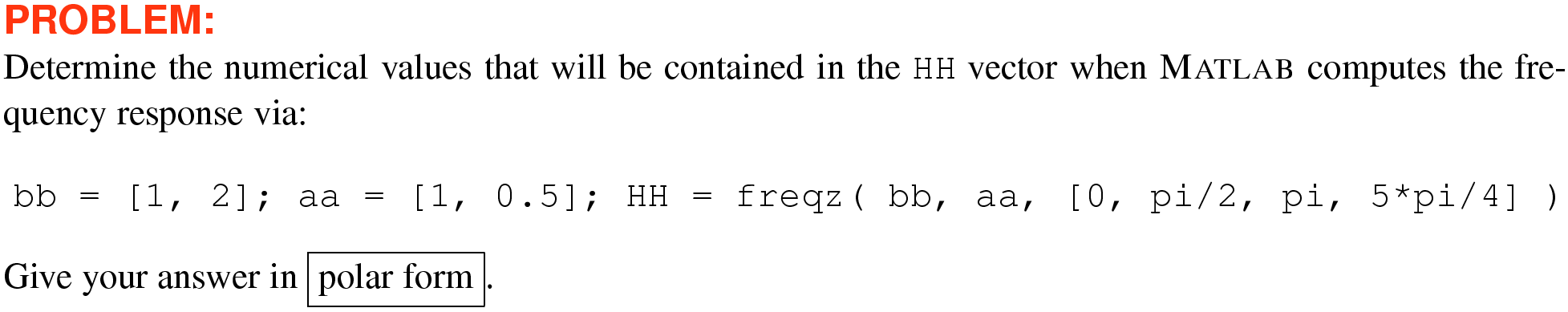
–126 Computing Frequency Response With MATLAB
Solution
10
–127 Find Poles and Zeros From System Functions
Solution
10
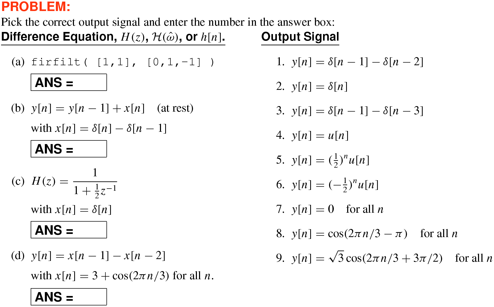
–128 Match Frequency Response to Difference Equation or Impulse Response
Solution
10
–129 Match System Function or Difference Equation to Output
Solution
10
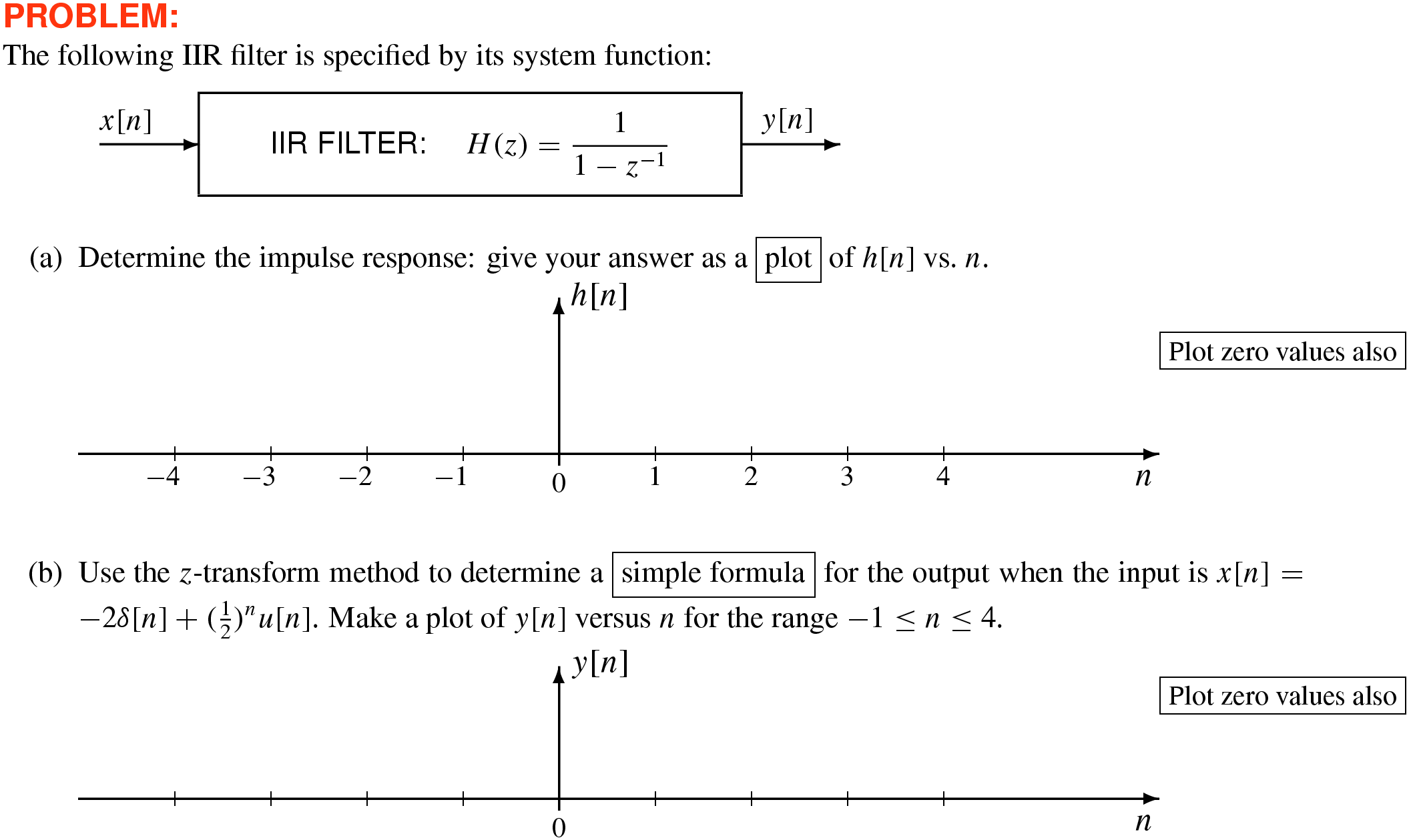
–130 Plot Output of IIR System Function
Solution
10
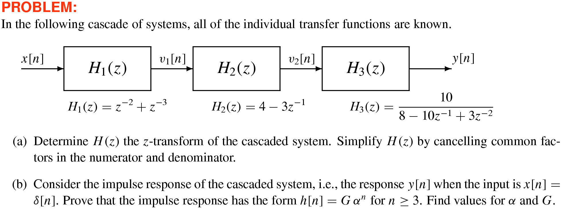
–131 Cascade of 3 LTI Systems ♦ \(H(z)\) ♦ Impulse Response
Solution
10
–132 Matching Impulse Response \(h[n]\) to \(H(z)\) or Difference Equation
Solution
10
–133 Matching Frequency Response to \(H(z)\) or Difference Equation
Solution
10
–134 Matching Impulse Responses
Solution
10
–135 Matching Frequency Responses
Solution
10
–136 Matching Pole-Zero Diagrams
Solution
10
–137 \(H(z)\) from IIR Difference Equation ♦ Poles & Zeros ♦ Output Signal
Solution
10
–138 Design IIR Filter \(H(z)\) to Synthesize \(y[n]\)
Solution
10
–139 MATLAB Functions: filter( ) & freqz( ) use Filter Coefficients
Solution
10
–140 Output Signal for IIR Difference Equation ♦ Finite-Length Input Signal
Solution
10
–141 Difference Equation from Poles & Zeros of \(H(z)\) ♦ Impulse Response
Solution
10
–142 Output Signal for IIR Difference Equation ♦ Finite-Length Input Signal
Solution
10
–143 Frequency Response from Pole-Zero Plot
Solution
10
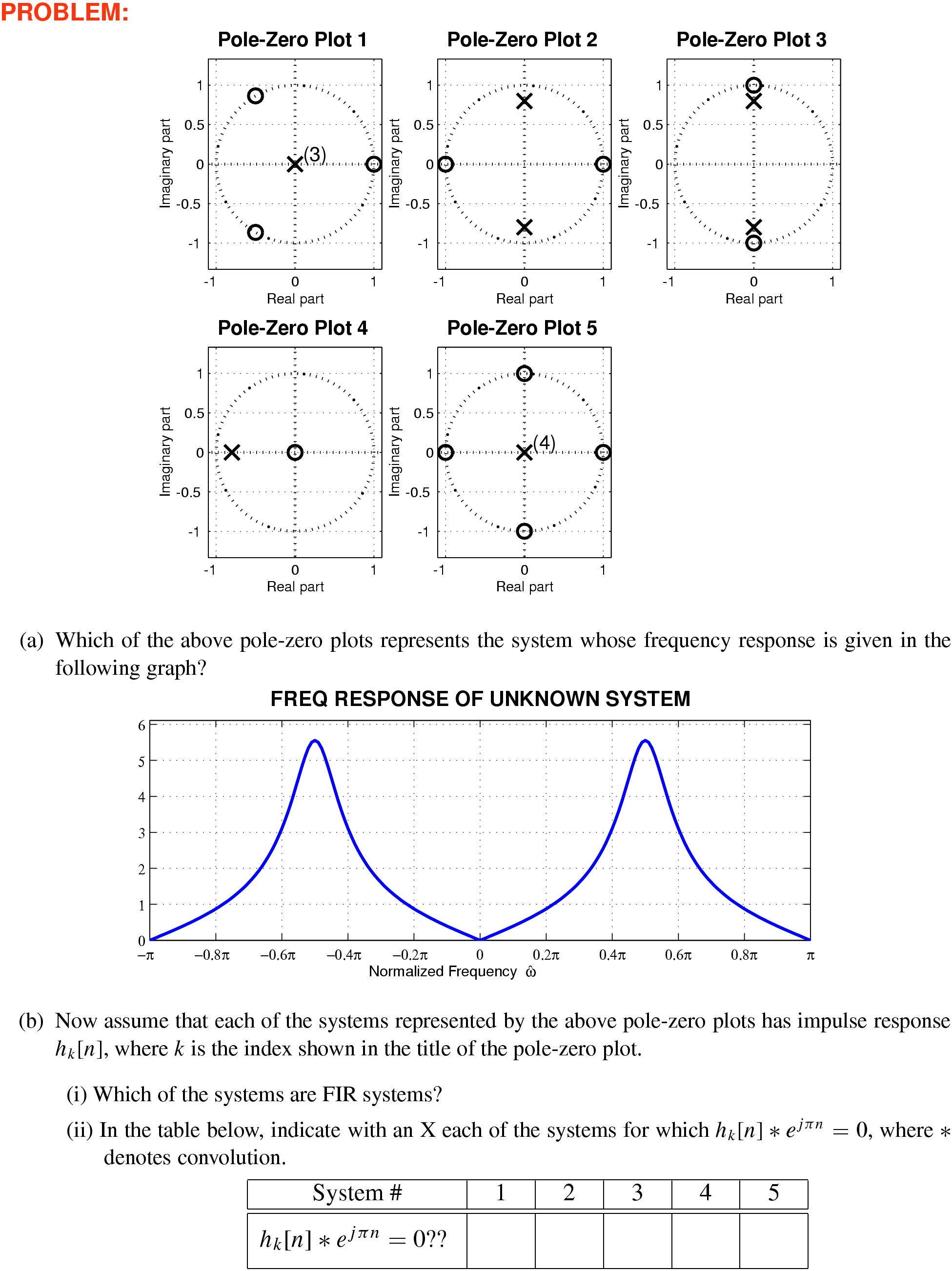
–144 Matching Pole-Zero Plots to Various \(H(z)\) and Difference Equations
Solution
10
–145 Matching Impulse Responses \(h[n]\) to Various \(H(z)\) and Difference Equations
Solution
10
–146 Matching Frequency Responses to Various \(H(z)\) and Difference Equations
Solution
10
–147 Design IIR Filter \(H(z)\) to Synthesize a Sinusoid ♦ D/C Reconstruction
Solution
10
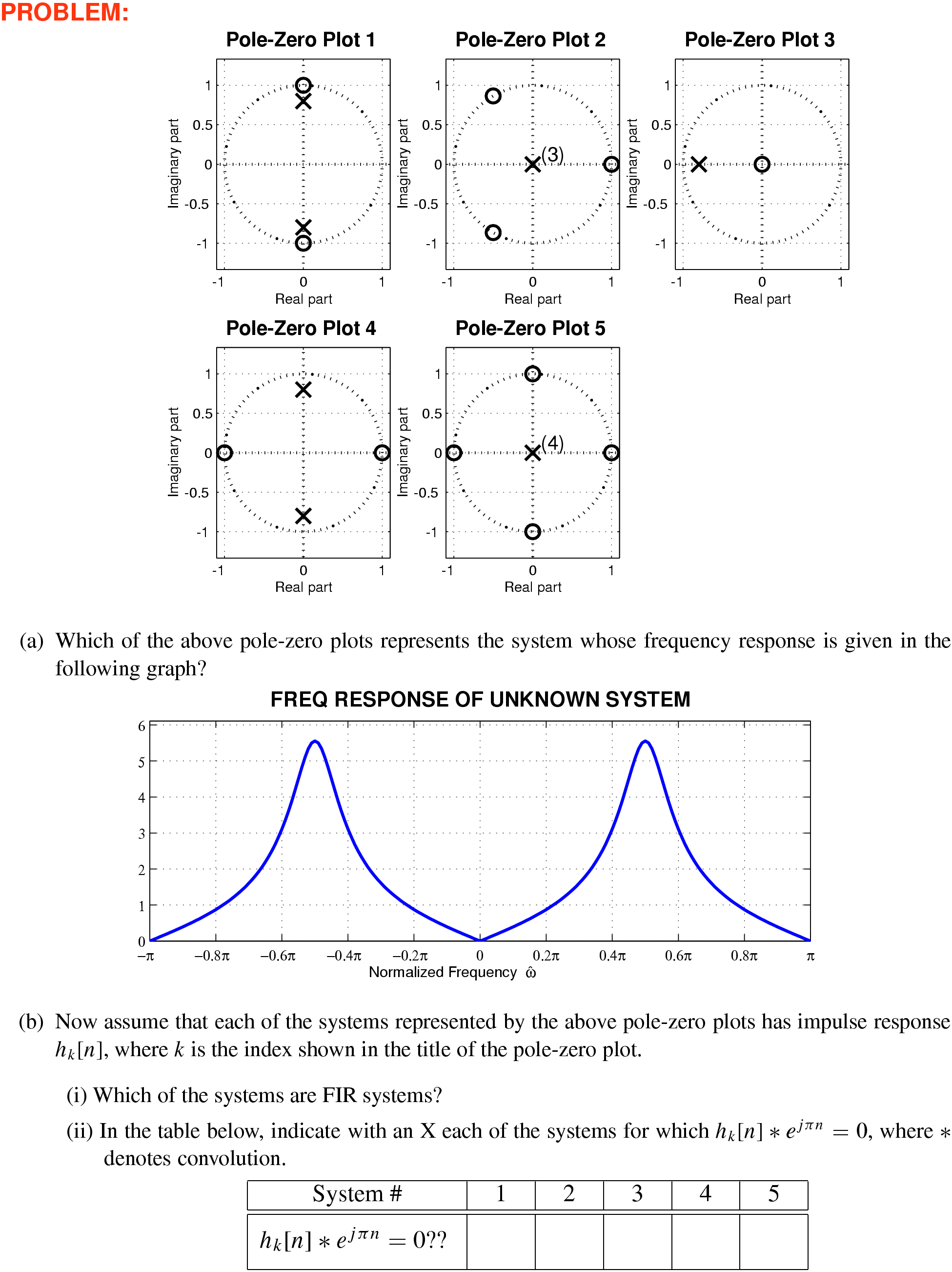
–148 Matching Pole-Zero Plots to Various \(H(z)\) and Difference Equations
Solution
10
–149 Matching Impulse Responses \(h[n]\) to Various \(H(z)\) and Difference Equations
Solution
10
–150 Matching Frequency Responses to Various \(H(z)\) and Difference Equations
Solution
10
–151 Impulse Response & Poles of IIR Filter Defined by MATLAB ♦ D/C Conversion
Solution
10
–152 Cascade of 3 LTI Systems ♦ \(H(z)\) ♦ Impulse Response
Solution
10
–153 Difference Equation from \(H(z)\) ♦ Frequency Response
Solution
10
–154 \(H(z)\) from IIR Difference Equation ♦ Poles & Zeros ♦ Output Signal
Solution
10
–155 Impulse Response of a 2nd-Order IIR Filter
Solution
10
–156 \(H(z)\) from IIR Difference Equation ♦ Frequency Response ♦ Poles & Zeros
Solution
10
–157 Difference Equation from \(H(z)\) ♦ Frequency Response ♦ Poles & Zeros
Solution
10
–158 \(H(z)\) from IIR Difference Equation ♦ Poles & Zeros
Solution
10
–159 Output Signal & Frequency Response for IIR Filter Defined by MATLAB Code
Solution
10
–160 Cascade of 3 LTI Systems ♦ \(H(z)\) ♦ Impulse Response ♦ Difference Equation
Solution
10
–161 Matching Frequency Responses to 2 Difference Equations
Solution
10
–162 Difference Equation and \(H(z)\) from Block Diagram of IIR Filter
Solution
10
–163 \(H(z)\) from Difference Equation
10
–164 Match Frequency Responses to Difference Equations
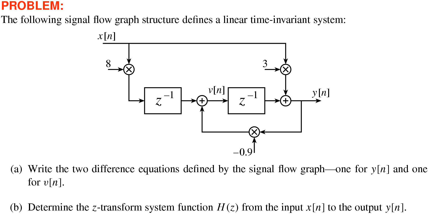
10
–165 Difference Equation from Signal Flow Graph
10
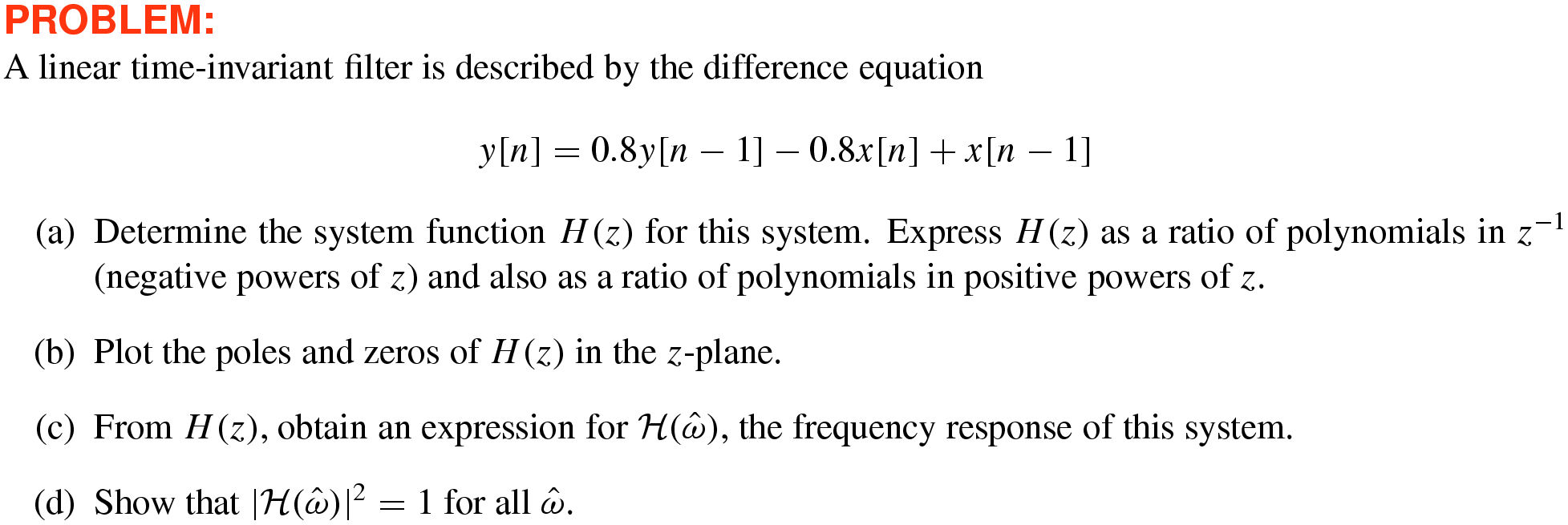
–166 \(H(z)\) from Difference Equation
10
–167 Damped Sinusoid Response of Second-Order Filter
10
–168 Response of Recursive Difference Equation
10
–169 \(H(z)\) for Recursive Difference Equation
10
–170 Frequency Response and Difference Equation from \(H(z)\)
10
–171 Match Impulse Responses to \(H(z)\) and Difference Equations
10
–172 Match Frequency Responses to \(H(z)\) and Difference Equations
10
–173 Poles and Zeros from Difference Equations and \(H(z)\)
10
–174 Impulse Response and \(H(z)\) for cascade of 3 systems
10
–175 Plot Output of IIR System Function
Solution
10
–176 System Functions and Frequency Response
Solution
10
–177 Matching Impulse Response \(h[n]\) to \(H(z)\) or Difference Equation
Solution
10
–178 Matching Frequency Response to \(H(z)\) or Difference Equation
Solution
10
–179 Matching Pole-Zero Plot to Difference Equation
Solution
10
–180 Difference Equation of Two Cascaded Filters
Solution
10
–181 Matching Impulse Response \(h[n]\) to \(H(z)\) or Difference Equation
Solution
10
–182 Plot Output of IIR System Function
Solution
10
–183 Matching Frequency Response to \(H(z)\) or Difference Equation
Solution
10
–184 Matching Pole-Zero Plot to Difference Equation
Solution
10
–185 System Functions and Frequency Response
Solution
10
–186 Difference Equation of Two Cascaded Filters
Solution
10
–187 Cascade of 3 LTI Systems ♦ \(H(z)\) ♦ Impulse Response
Solution
10
–188 Matching Frequency Response to \(H(z)\) or Difference Equation
Solution
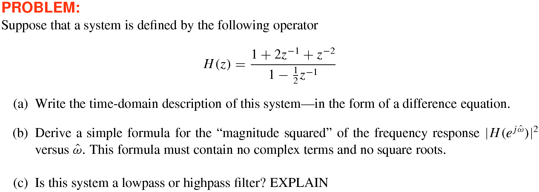
10.2
–189 \(H(z)\) to \(H(\hat\omega)\) & Difference Equation
Solution
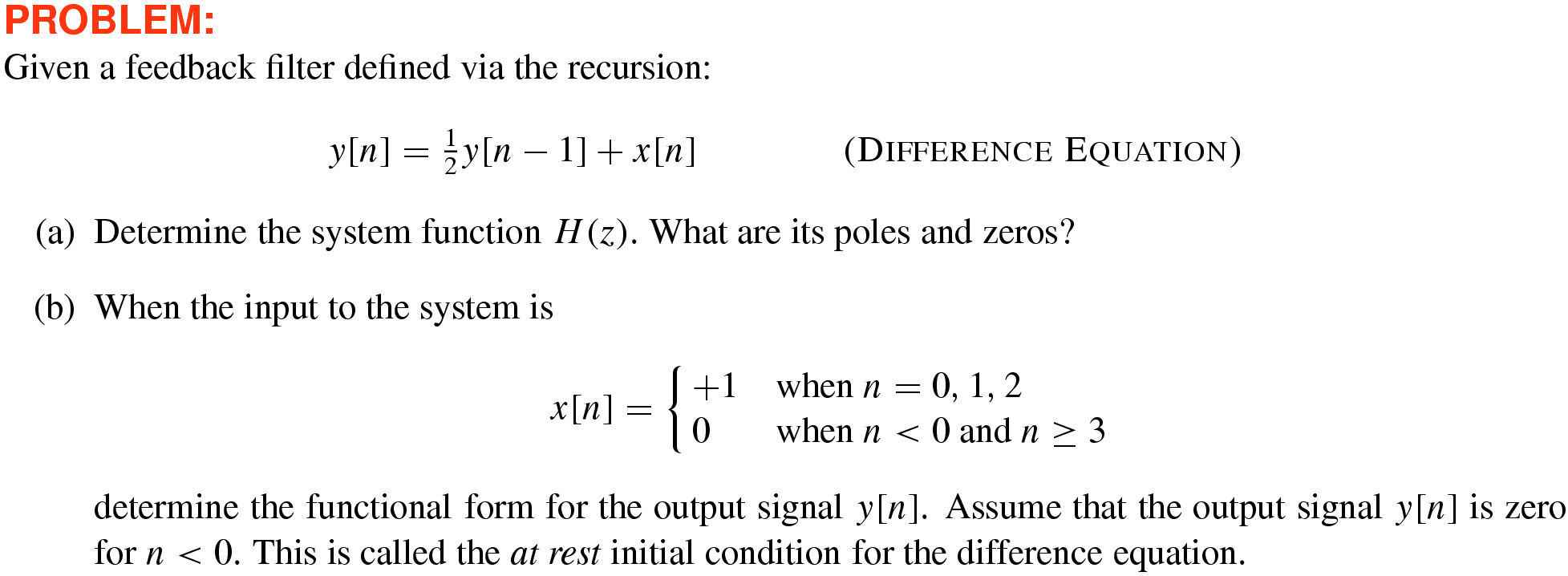
10.6
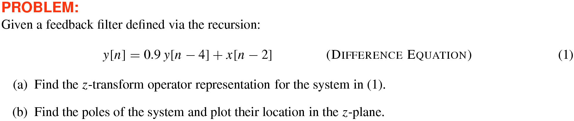
–190 \(H(z)\) for Feedback Filter
Solution
10.7
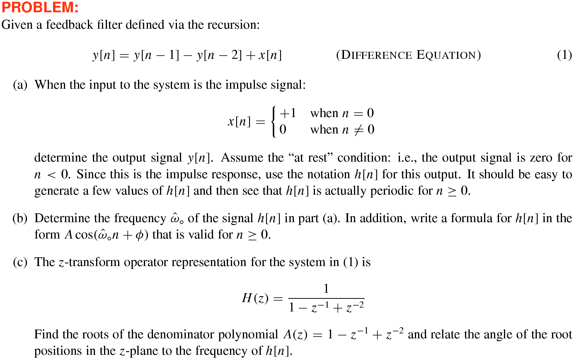
–191 \(H(z)\) for Feedback Filter
Solution
10.8
–192 \(H(z)\) for Feedback Filter
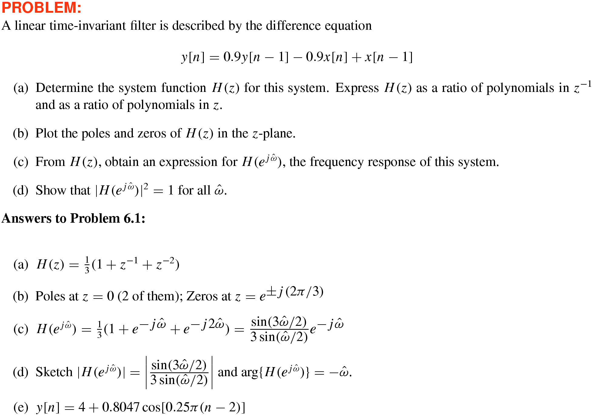
Solution
10.13
–193 Matching Pole-Zero Plots
Solution
10.14
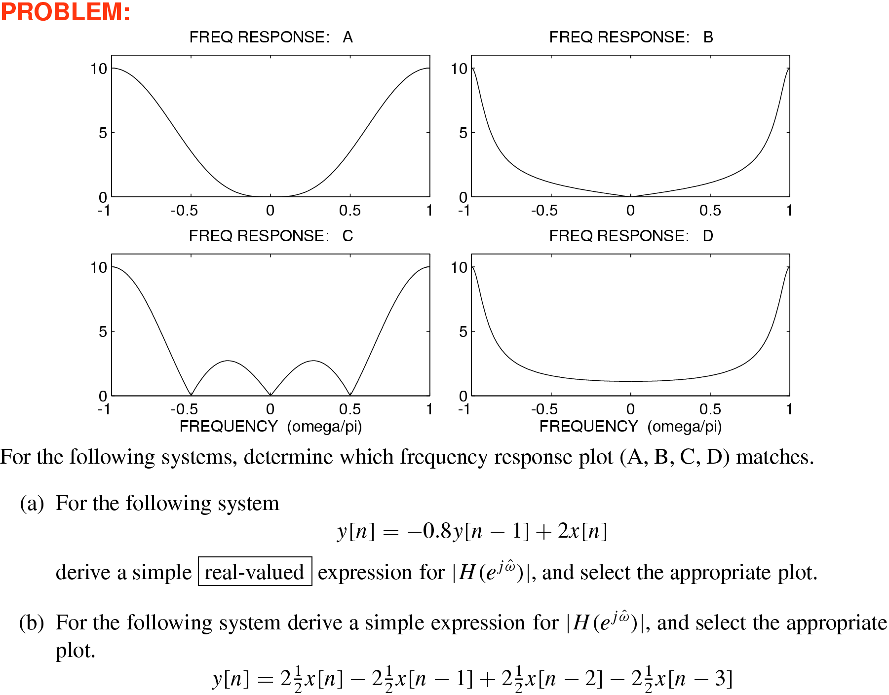
–194 Matching Frequency Response
Solution
10.16
–195 Matching \(z\mbox{-}\)Plane & \(H(\hat\omega)\)
Solution
10.17
–196 Matching \(z\mbox{-}\)Plane & \(h[n]\)
Solution
10.21
–197 Cascade of 2 Systems: FIR & Feedback
Solution
10.22
–198 Synthesize Feedback Filter
Solution