DSP FIRST 2e
Examples
93
A
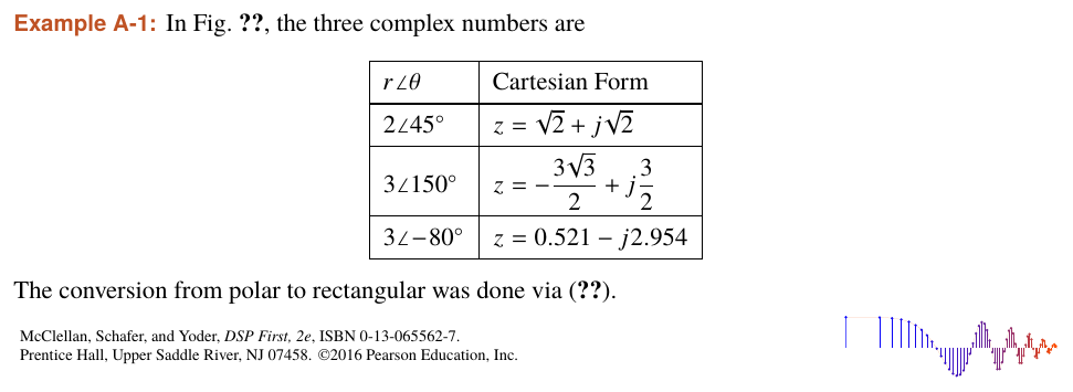
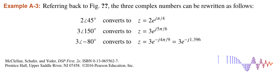
.1: Polar to Rectangular
A
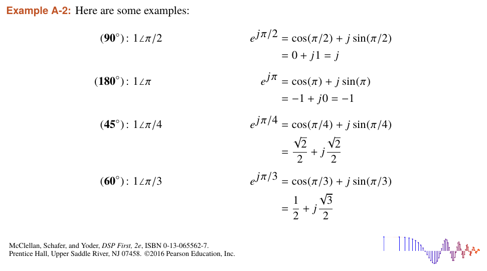
.2: Euler’s Formula
A
.3: Degrees to Radians
A
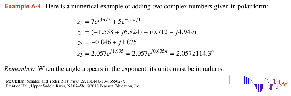
.4: Adding Polar Forms
A
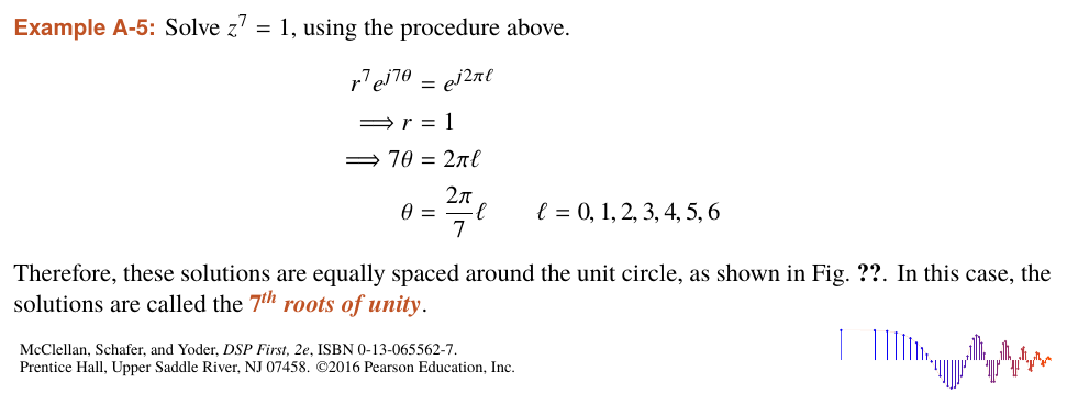
.5: 7th Roots of Unity
C
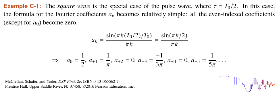
.1: Square Wave
C
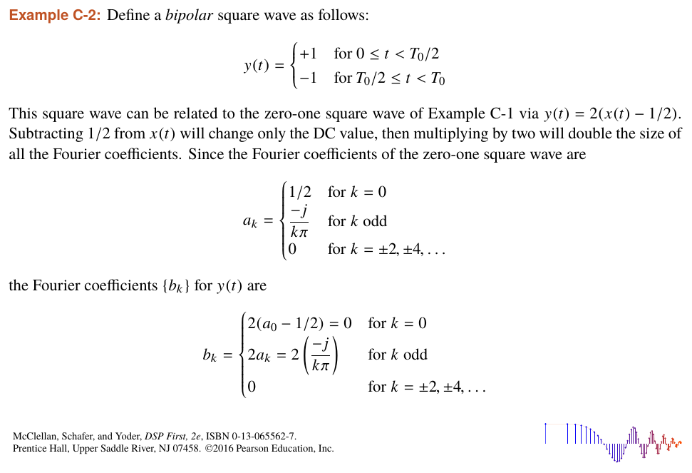
.2: New Square Wave
C
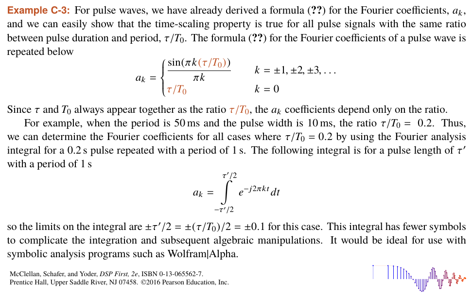
.3: Time-Scaling Pulse Waves
C
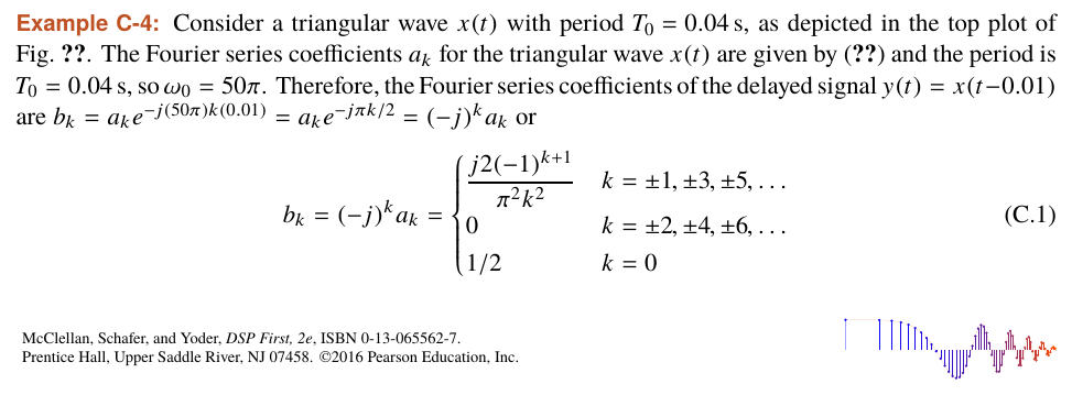
.4: Delayed Triangular Wave
C
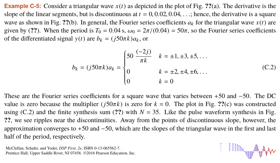
.5: Differentiated Triangular Wave
C
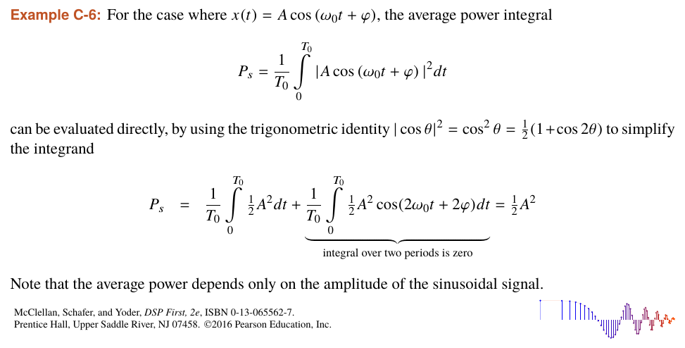
.6: Average Power of a Sinusoid
2
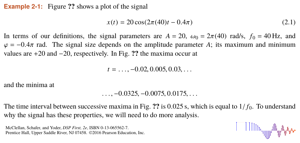
.1: Plotting Sinusoids
3
.1: Two-Sided Spectrum
3
.10: Average Power in Sinusoid
3
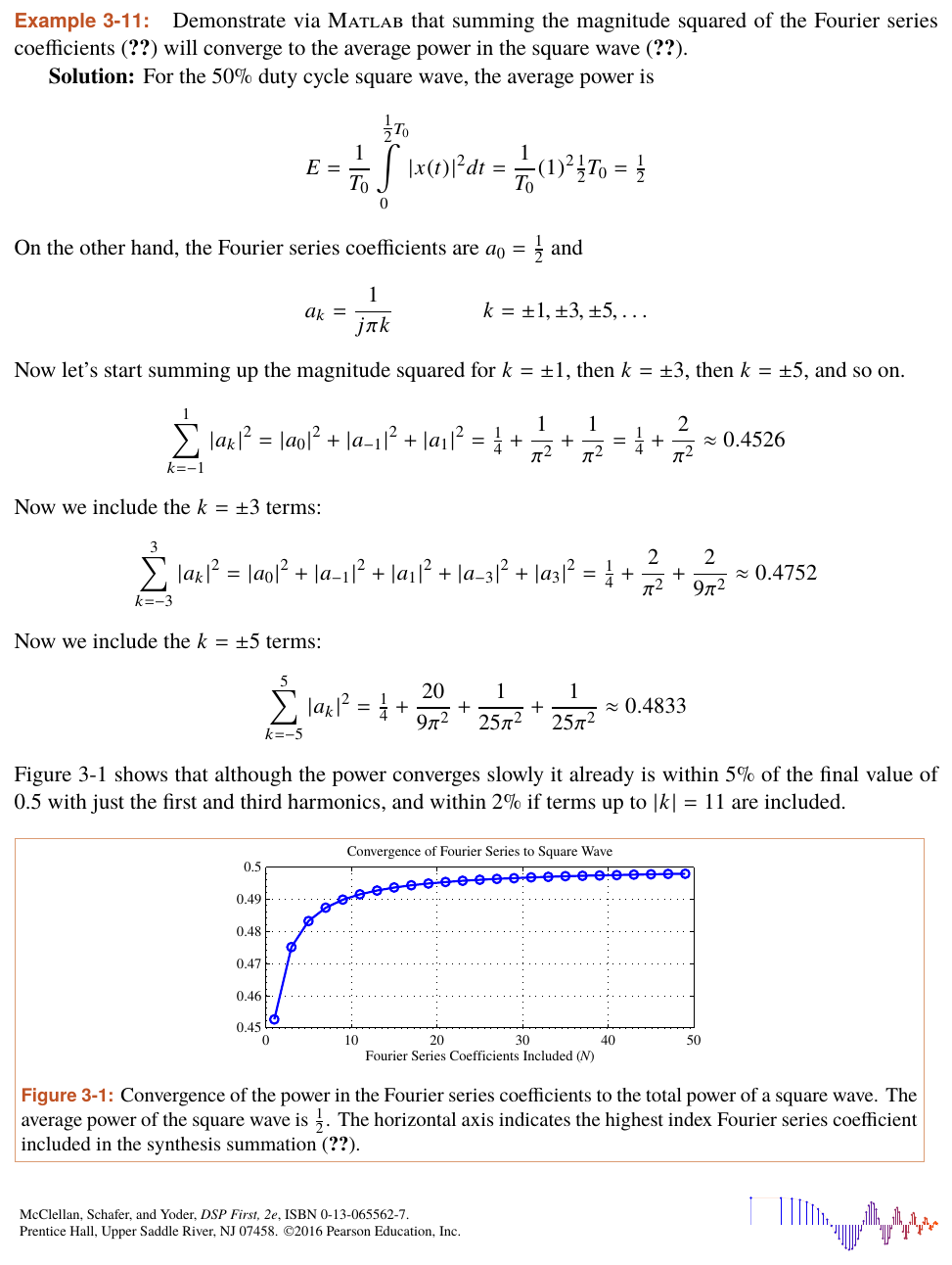
.11: Average Power in Square Wave
3
.12: Synthesize a Chirp Formula
3
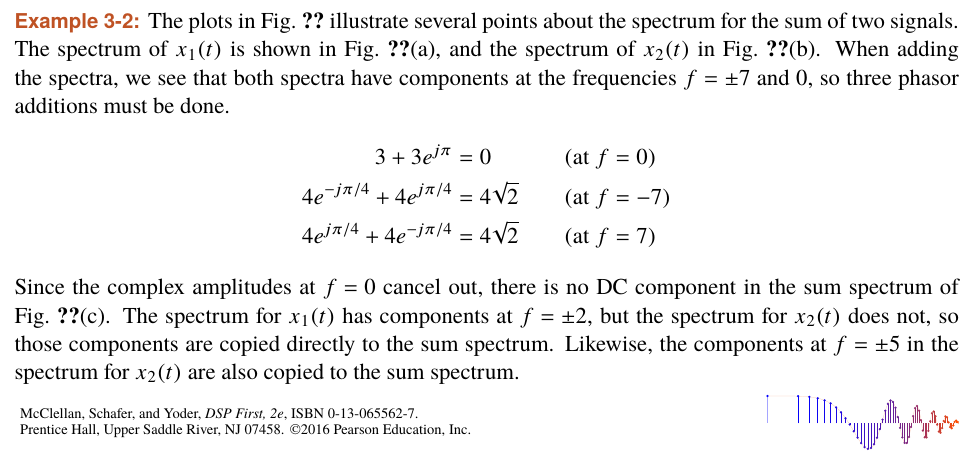
.2: Adding Spectra
3
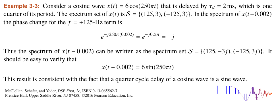
.3: Delayed Cosine
3
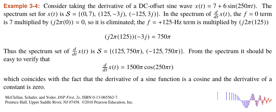
.4: Derivative of Sine plus DC
3
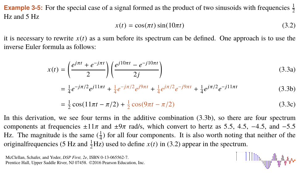
.5: Spectrum of a Product Signal
3
.6: Decreasing the Frequency Difference, \(f_\Delta\)
3
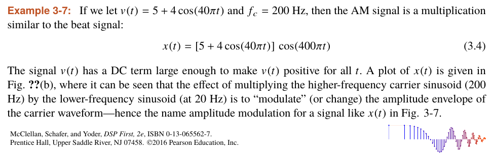
.7: Amplitude Modulation
3
.8: Fundamental Period T0
3
.9: Calculating F0
5
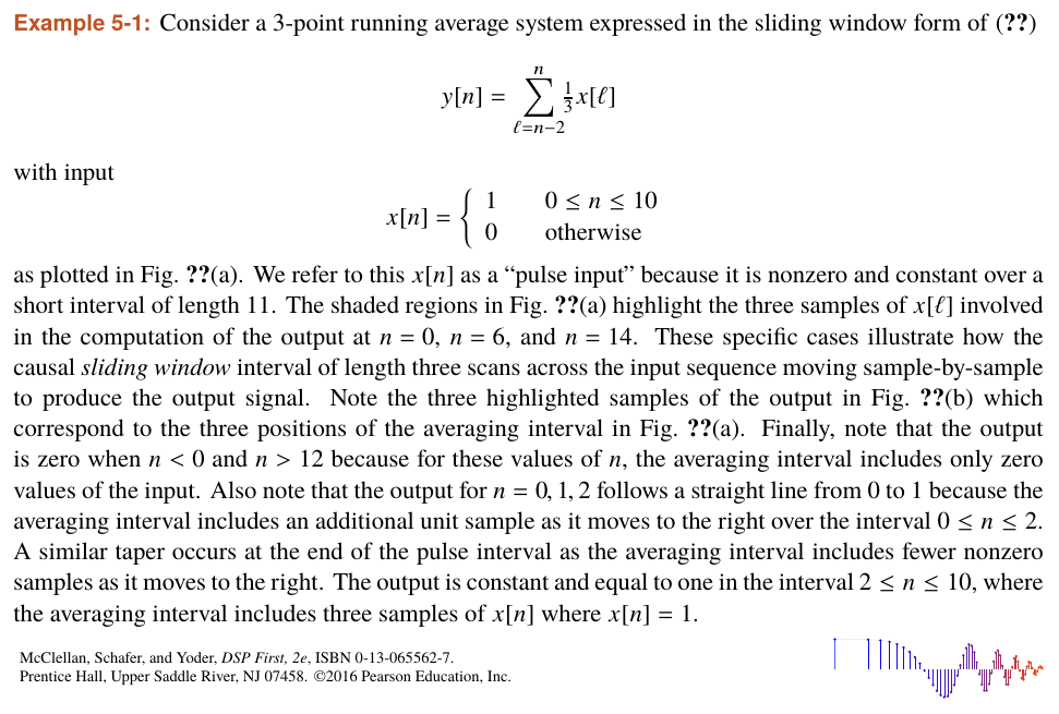
.1: Pulse Input to 3-Point Running Average
5
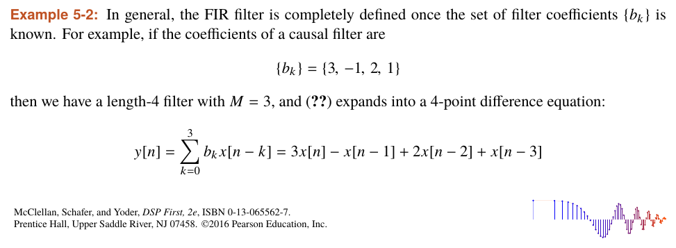
.2: FIR Filter Coefficients
5
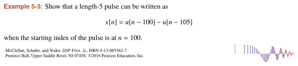
.3: Pulse as the Difference of Two Shifted Unit Steps
5
.4: Impulse Response of Cascaded Systems
6
.1: Formula for the Frequency Response
6
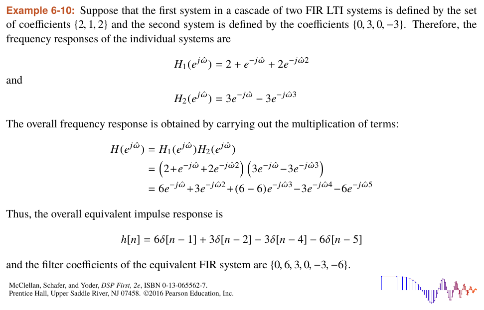
.10: Frequency Responses in Cascade
6
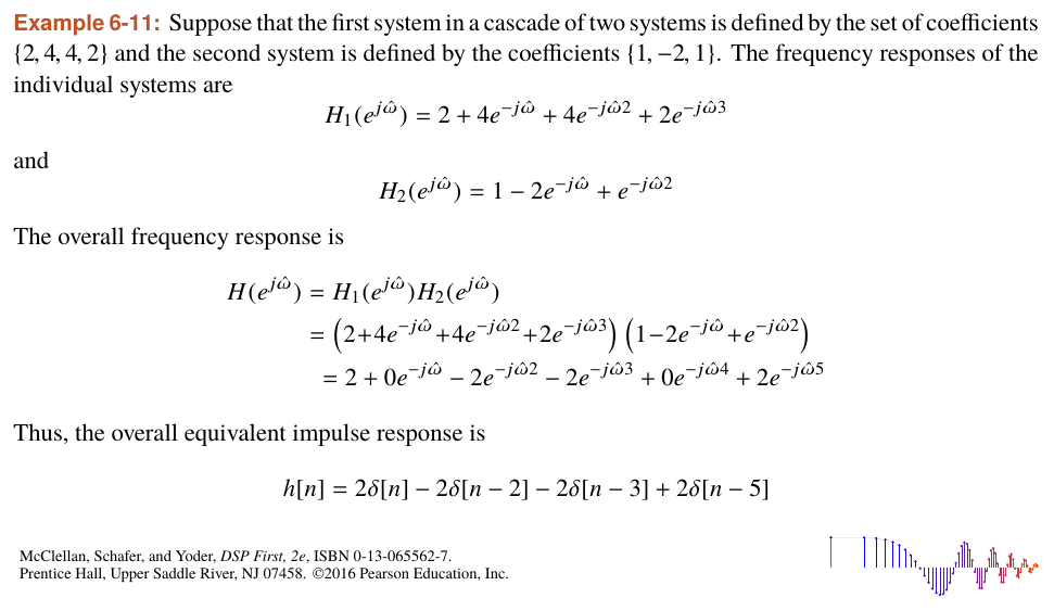
.11: Cascade
6
.12: Cascade
6
.13: Time Delay of FIR Filter
6
.2: Complex Exponential Input
6
.3: Cosine Input
6
.4: Three Sinusoidal Inputs
6
.5: Steady-State Output
6
.6: \(h[n]\) ←→ \(H(e^{j\hat\omega})\)
6
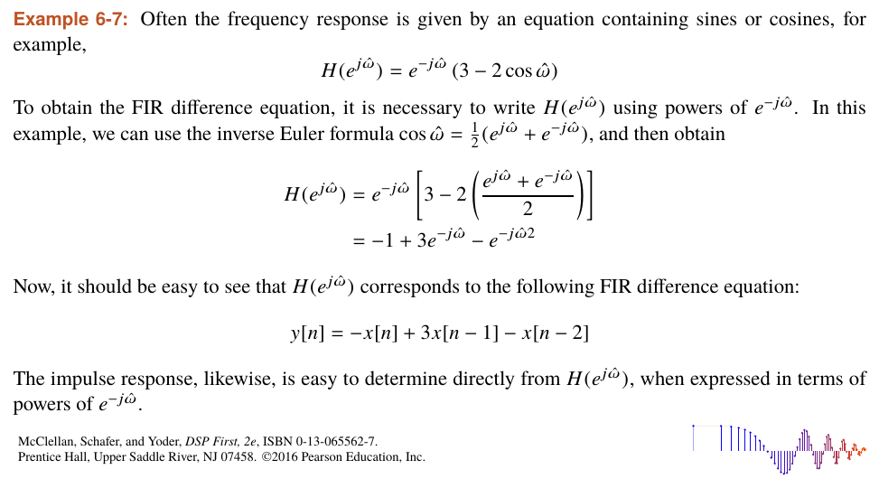
.7: Difference Equation from \(H(e^{j\hat\omega})\)
6
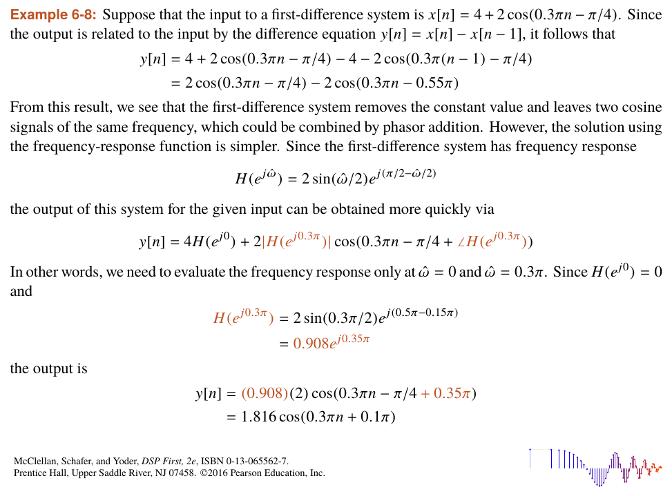
.8: First-Difference Removes DC
6
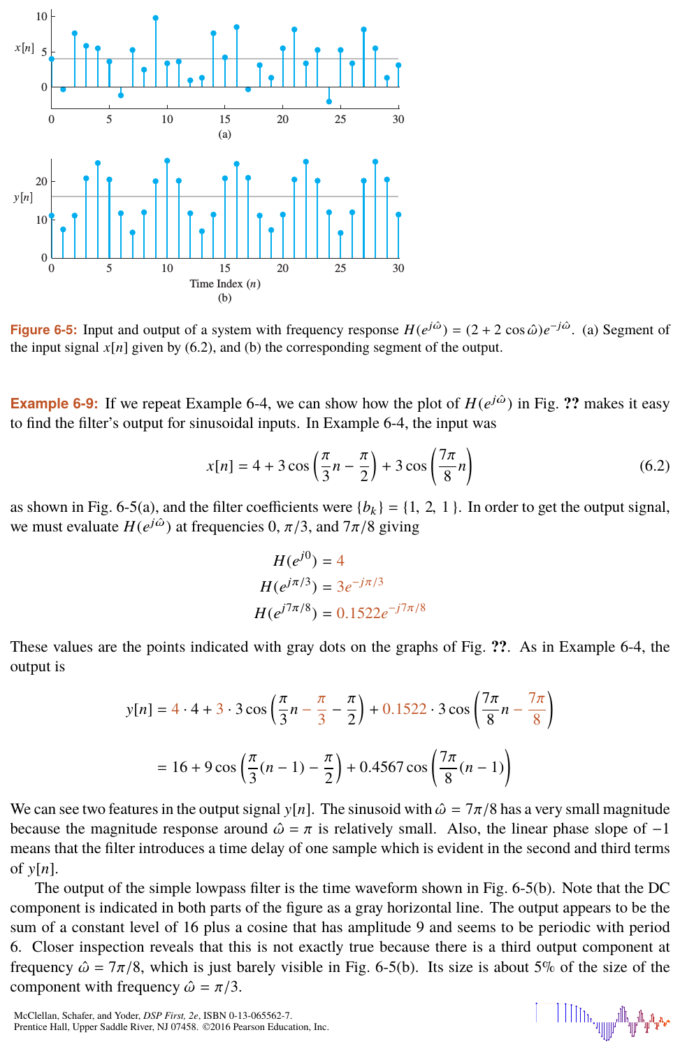
.9: Lowpass Filter
7
.1: DTFT of an FIR Filter
7
.2: DTFT of a Complex Exponential?
7
.3: Delayed Sinc Function
7
.4: Frequency Response of Delay
7
.5: Energy of the Sinc Signal
7
.6: Ideal Lowpass Filtering
7
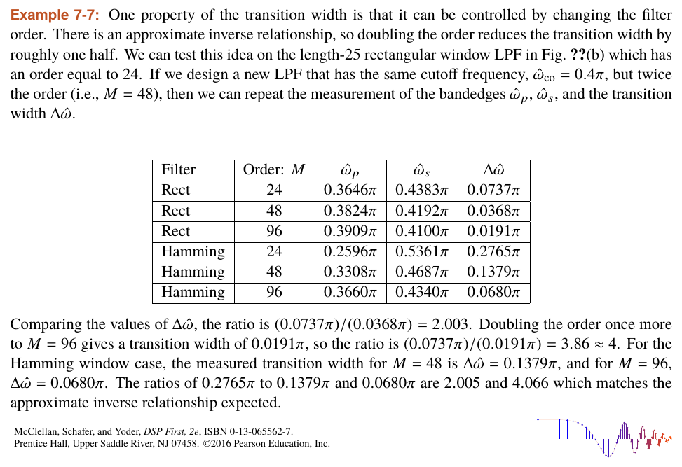
.7: Transition Width versus Filter Order
8
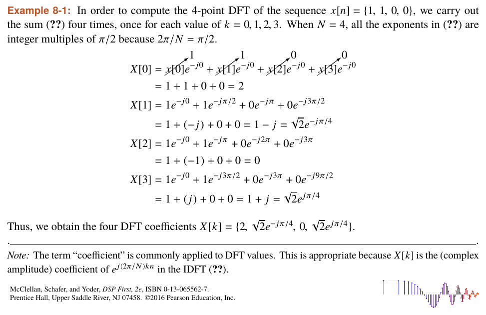
.1: Short-Length DFT
8
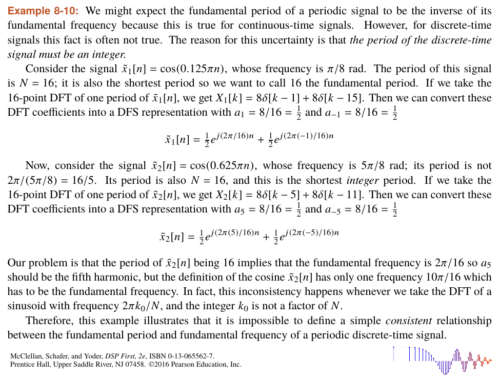
.10: Period of a Discrete-Time Sinusoid
8
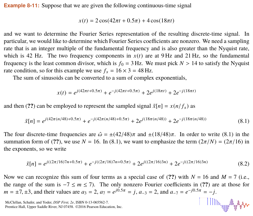
.11: Fourier Series of a Sampled Signal
8
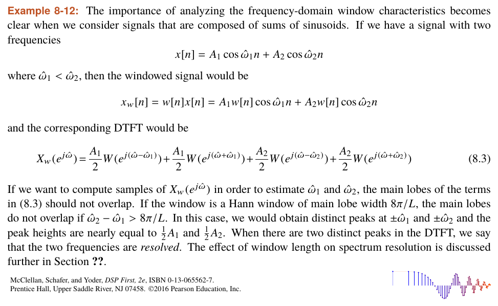
.12: Sum of Two Sinusoids
8
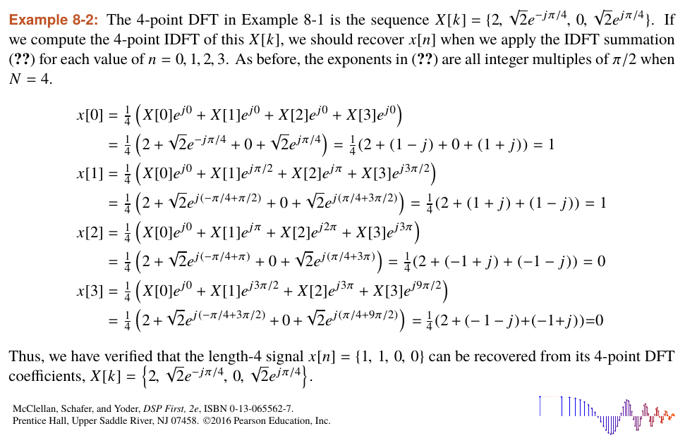
.2: Short-Length IDFT
8
.3: DFT Symmetry
8
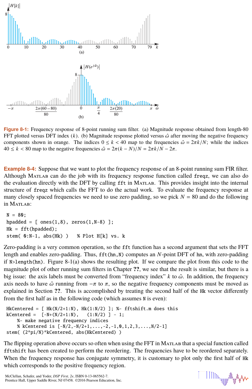
.4: Frequency Response Plotting with DFT
8
.5: DFT of Shifted Impulse
8
.6: Modulo- N Arithmetic
8
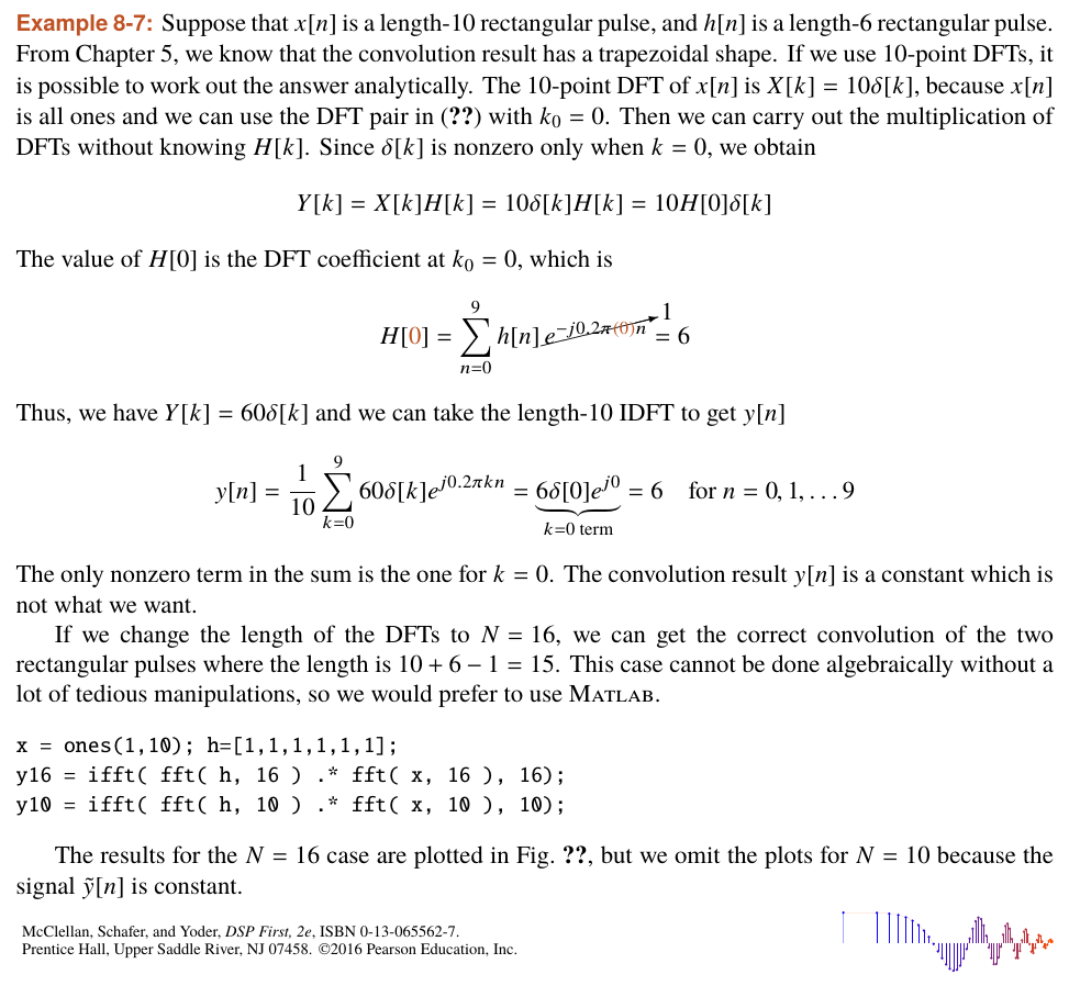
.7: Convolution of Pulses
8
.8: Synthesize a Periodic Signal from DFS
8
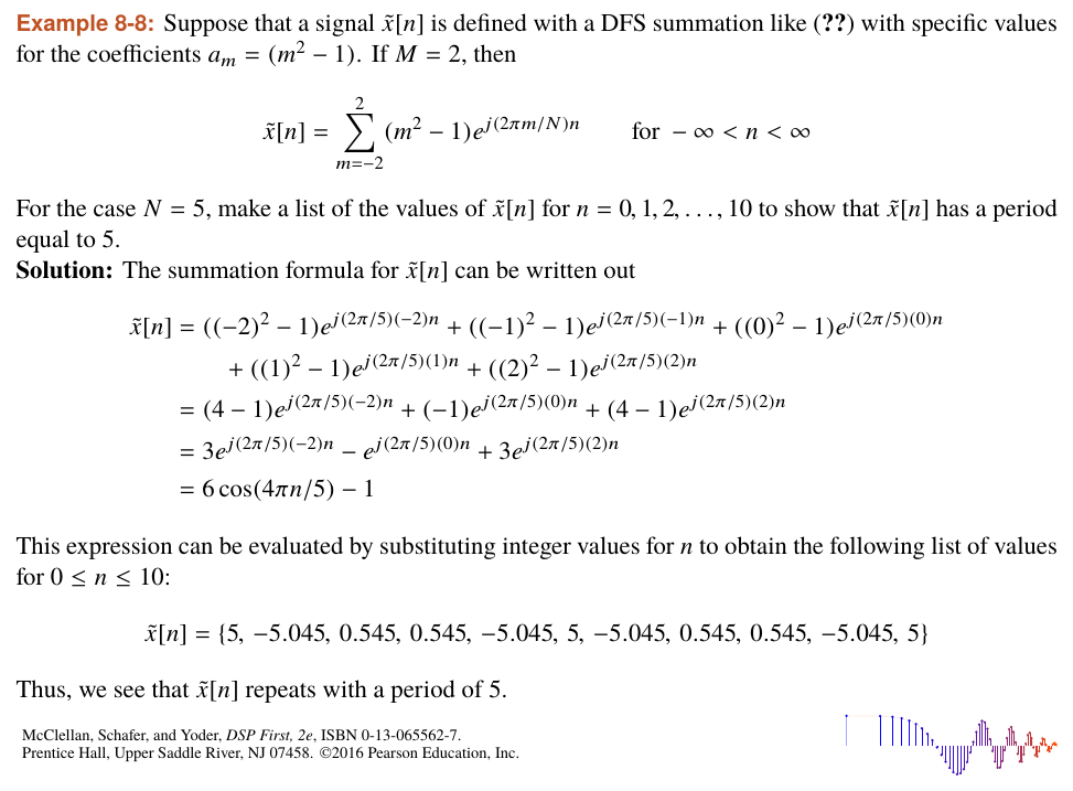
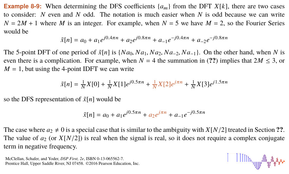
.9: Conjugate Symmetry of DFS Coefficients
9
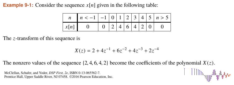
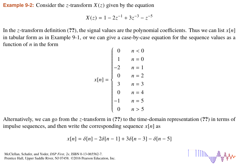
.1: \(z\mbox{-}\)Transform of a Signal
9
.10: Nulling Signals with Zeros
9
.11: \(H(e^{j\hat\omega})\) from \(H(z)\)
9
.2: Inverse \(z\mbox{-}\)Transform
9
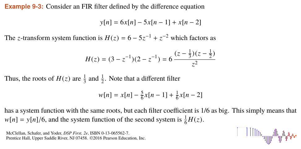
.3: Zeros of System Function
9
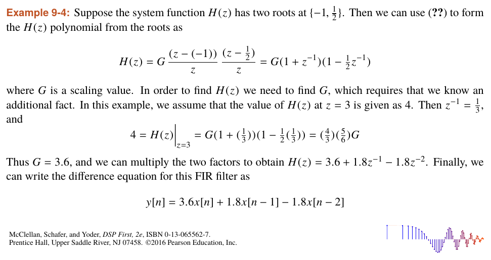
.4: Difference Equation from Roots of \(H(z)\)
9
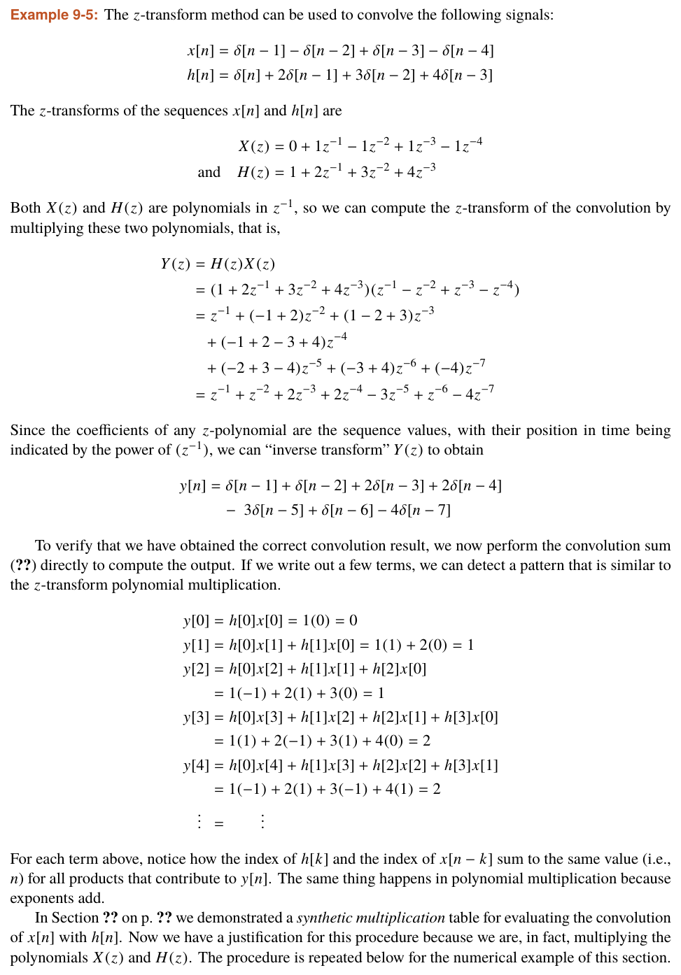
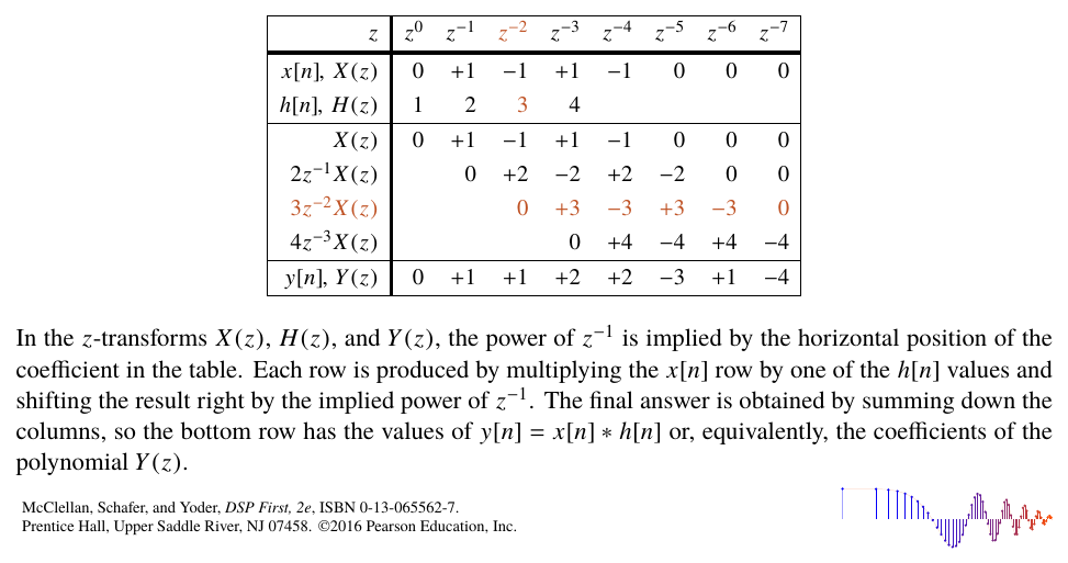
.5: Convolution via \(H(z)\)X (z)
9
.5a:
9
.6: \(H(z)\) for Cascade
9
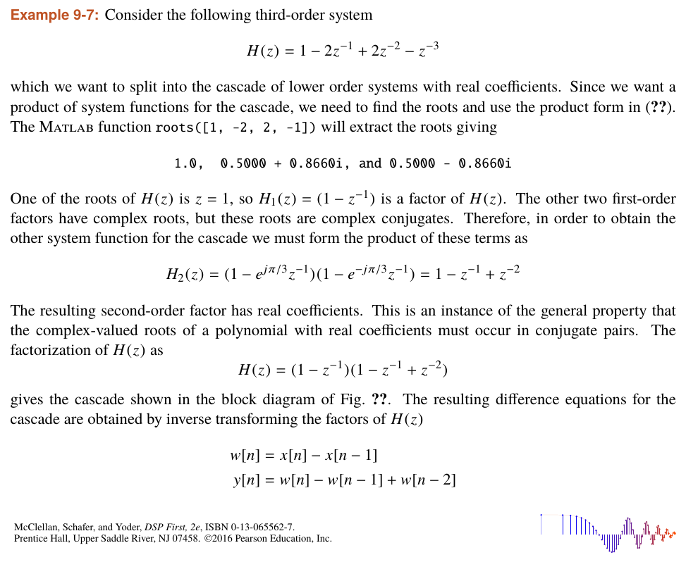
.7: Split \(H(z)\) into a Cascade
9
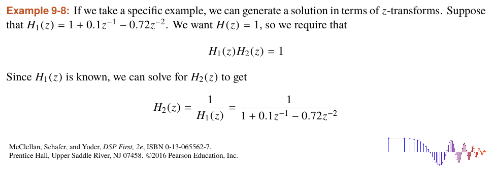
.8: Deconvolution
9
.9: Moving from \(\hat\omega\)
10
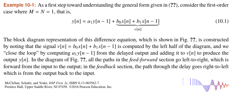
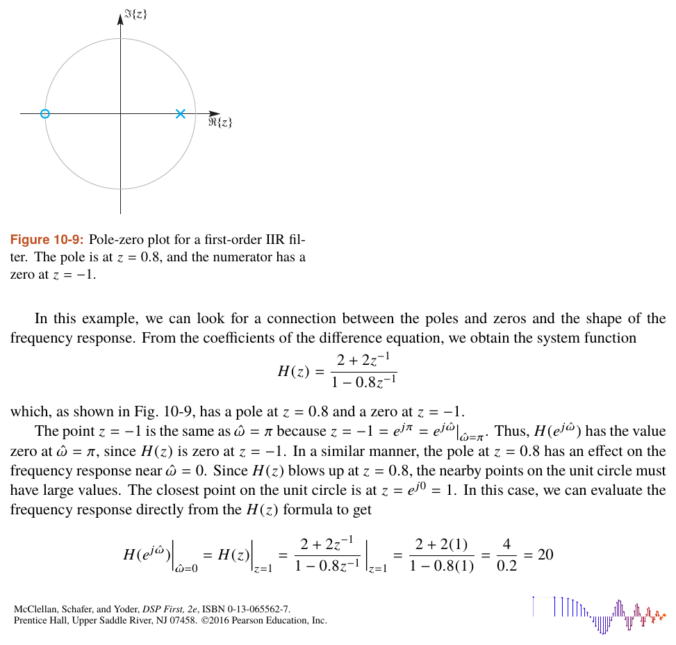
.1: IIR Block Diagram
10
.10: Plot \(H(e^{j\hat\omega})\) via MATLAB
10
.10a:
10
.11: Inverse \(z\mbox{-}\)Transform
10
.12: Long Division and Partial Fractions
10
.13: Transient and Steady-State Responses
10
.14: Complex Poles
10
.15: Second-Order System Real Poles
10
.16: Second-Order System
10
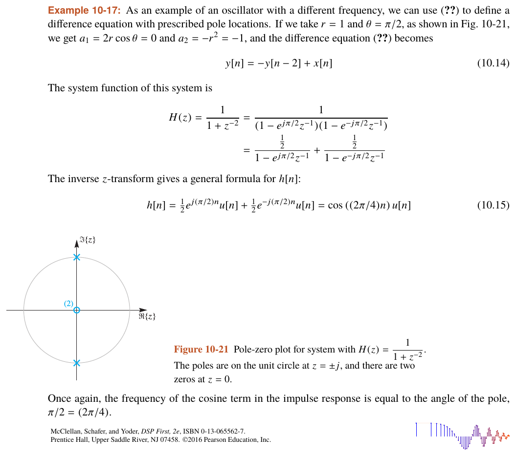
.17: Poles on Unit Circle
10
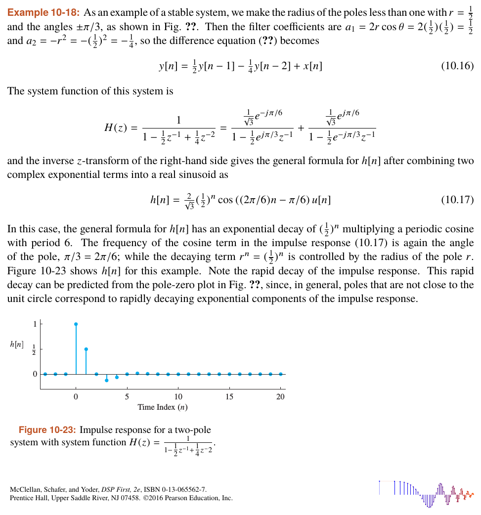
.18: Stable Complex Poles
10
.19: Frequency Response of a Second-Order System
10
.2: Impulse Response
10
.20: MATLAB for \(H(e^{j\hat\omega})\)
10
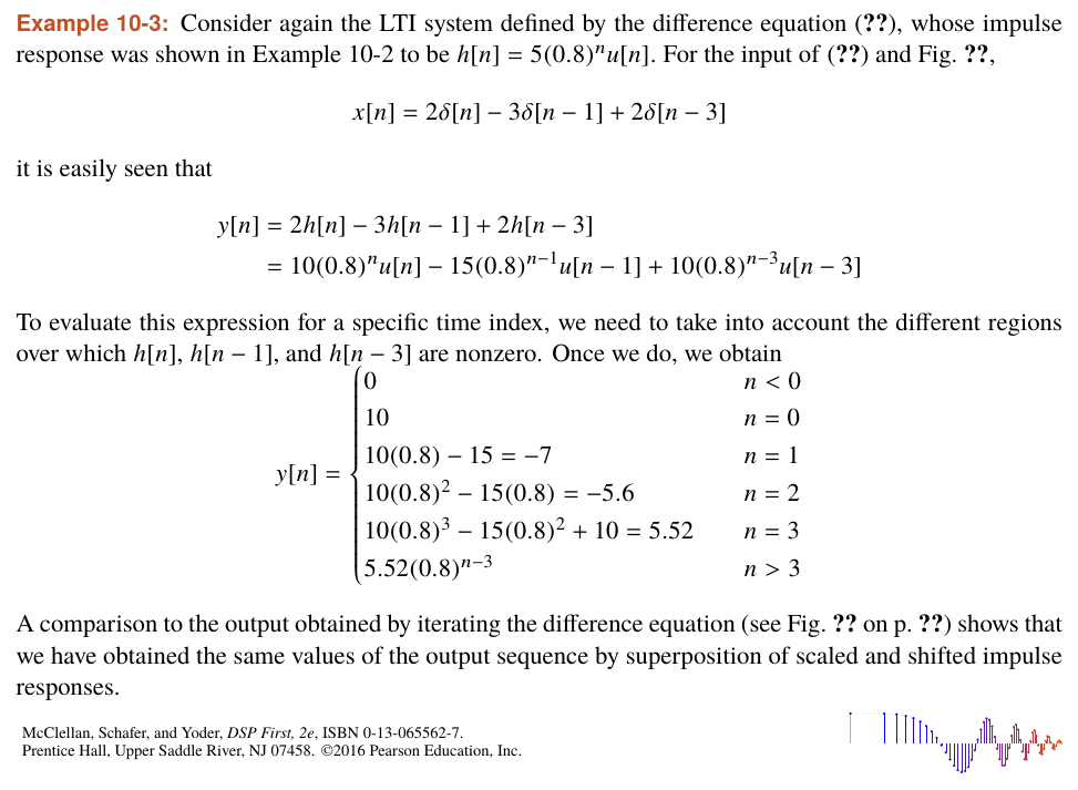
.3: IIR Response to General Input
10
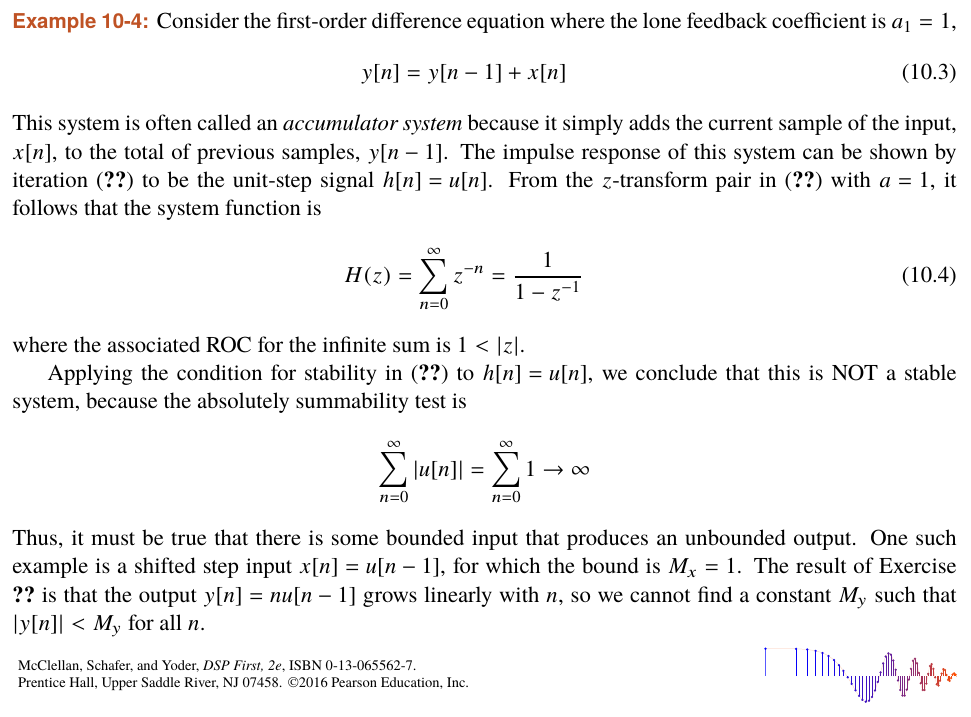
.4: Unstable System
10
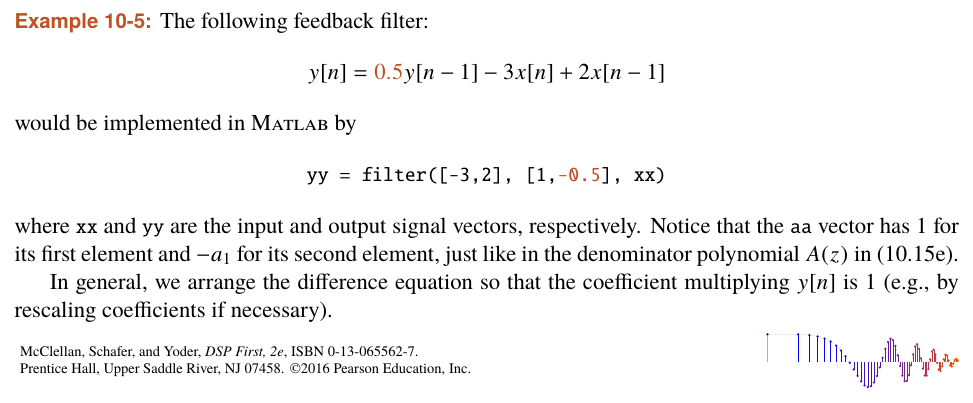
.5: MATLAB for IIR Filter
10
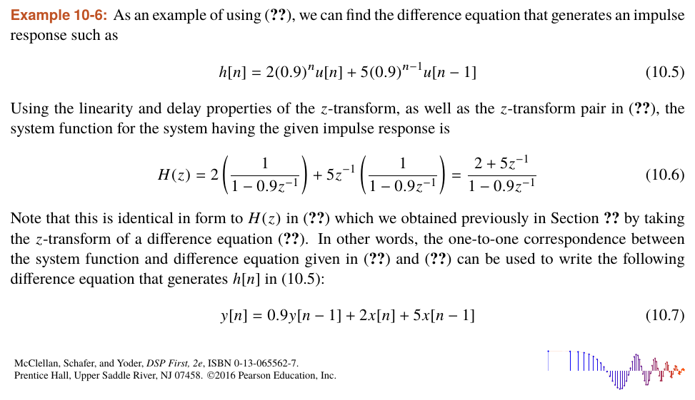
.6: \(H(z)\) from Impulse Response
10
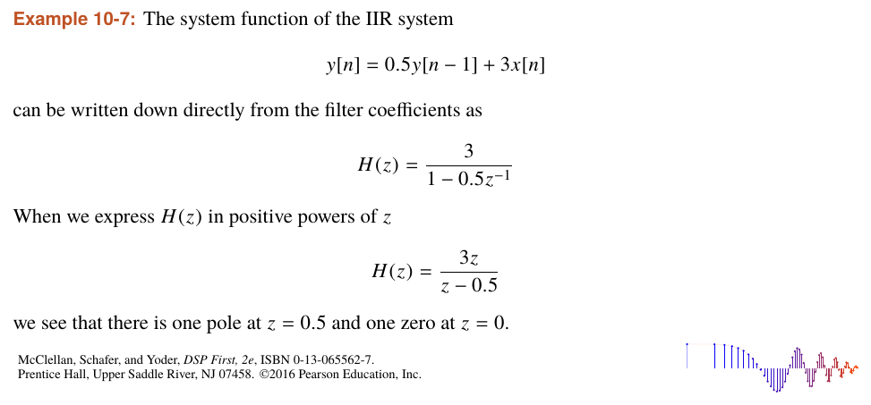
.7: Find Poles and Zeros
10
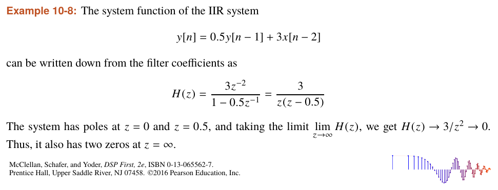
.8: Zeros at \(z=\infty\)
10
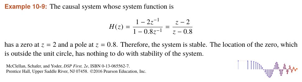
.9: Stability from Pole Location